Functions of several variables OLD

Continuity

Before we consider continuity of functions of several variables, let's recall how the issue is handled in Calc1 as there is a subtle difference.

Problem. For the function $f(x) = \sqrt{x}$ discuss continuity.

• at $x = 0$, $f$ is not continuous. However it is right-continuous at $\{0 \}$ as $x = 0$ is the end point of $D(f)$.
• at $x > 0$, $f$ is continuous.
• for $x < 0$, $f$ is undefined.

Thus $f$ is continuous on on $( 0, {\infty} )$ or continuous in the extended sense on $[ 0, {\infty} )$.

Recall the definition. A function $f: {\bf R} {\rightarrow} {\bf R}, f(x) = y,$ is continuous at point $a {\in} {\bf R}$ if for any ${\epsilon} > 0$ there is a ${\delta} > 0$ such that

$$| x - a | < {\delta} \rightarrow | f(x) - f(a) | < {\epsilon}.$$

Note that the definition implicitly assumes that $x, a {\in}$ $D(f)$.

How does the definition change in the $n$-dimensional case?

Definition. A function $f: {\bf R}^n {\rightarrow} {\bf R}, f(x) = y,$ is continuous at point $a {\in} D(f)$ if for any ${\epsilon} > 0$ there is a ${\delta} > 0$ such that

$$|| x - a || < {\delta} {\rm \hspace{3pt} and \hspace{3pt}} x {\in} D(f) \rightarrow || f(x) - f(a) || < {\epsilon}.$$

First, we have replaces the absolute value with the norm. This simply reflect the way we measure "closeness" in ${\bf R}$ versus in ${\bf R}^n$ (see Continuous functions).

Second, $x$ is required to be in the domain of $f$. This makes a difference. With the new definition, $\sqrt{x}$ is continuous on $[ 0, {\infty} )$ (verify). Thus one-side continuity is no longer an issue.

Now for ${\rm dim \hspace{3pt}} > 1$.

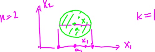
Example. Consider $f( x, y ) = ( x + y )^{\frac{1}{2}}, D(f) = \{ ( x, y ): x + y \geq 0 \}.$ Without actually verifying the definition, we see that the function is continuous on the whole domain - the half-plane including the border.

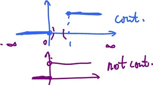
Example. Let $f(x) = 0$ if $x \leq 0, f(x) = 1$ if $x \geq 1.$

Is $f$ continuous? Yes! It is surprising, but since the domain is "disconnected", the function can't be (unlike the second example on the right).

Example. Let $f(x) = c$ a constant function. Then $|| f(x) - f(a) || = || c - c || = 0 < {\epsilon}$, so $f$ is continuous.

Theorem. Let $f: {\bf R}^n {\rightarrow} {\bf R}, f_k(x) = x_k,$ be the projection, where $x = ( x_1, ..., _n ).$ Then f is continuous.

(For example, if $n = 3, f_2 ( 1, 5, 7 ) = 5$.)

Proof. Consider $f_k(x) = a_k,$ where $a = ( a_1, ..., a_n ).)$

In order to show this, we have to find ${\delta}$ for a given ${\epsilon} > 0$. We hence want to show that for

$$|| x - a || < {\delta} $$

it follows that

$$| f_k(x) - f_k(a) | = | x_k - a_k | < {\epsilon}.$$

We rewrite $( ( x_1 - a_1 )^2 + ( x_2 - a_2 )^2 + ... )^{\frac{1}{2}} < {\delta},$ and $( ( x_1 - a_1 )^2 + ( x_2 - a_2 )^2 + ... )^{\frac{1}{2}} \geq ( ( x_k - a_k )^2 )^{\frac{1}{2}} = | x_k - a_k | < {\epsilon}.$

Choose ${\delta} = {\epsilon}$. Then if $$( ( x_1 - a_1 )^2 + ( x_2 - a_2 )^2 + ... )^{\frac{1}{2}} < {\delta} = {\epsilon},$$

then $$| x_k - a_k | < {\epsilon}.$$

For more see Continuity of functions of several variables.

Continuity under algebraic operations

Let's create new functions from old, using $+, -, \cdot, /, \circ$, and see how this affect continuity.

Theorem (Sum). If $f, g: {\bf R}^n {\rightarrow} {\bf R}$ are continuous at $x = a$, then so is $f + g$.

Proof. Let $h = f + g.$ We want to show that for every ${\epsilon} > 0$, there is a ${\delta} >0$ such that

$$| x - a | < {\delta}, x {\in} D(h) \rightarrow | h(x) - h(a) | < {\epsilon}.$$

Let's write the definition of continuity twice - for $f$ and $g$. As it turns out, choosing $\frac{\epsilon}{2}$ is preferable in order to get from these to the one above.

1. there is a ${\delta}_1 > 0$ such that $| x - a | < {\delta}_1, x {\in} D(f) \rightarrow | f(x) - f(a) | < \frac{\epsilon}{2},$
2. there is a ${\delta}_2 > 0$ such that $| x - a | < {\delta}_2, x {\in} D(g) \rightarrow | g(x) - g(a) | < \frac{\epsilon}{2}.$

Let ${\delta} = {\rm min}( {\delta}_1, {\delta}_2 ). $ Then ${\delta}_1, {\delta}_2 \leq {\delta}.$

Hence we can re-write the above two definitions as follows:

there is ${\delta} > 0$ such that $| x - a | < {\delta}, x {\in} D(f) \cap D(g) = D(h) \rightarrow | f(x) - f(a) | < \frac{\epsilon}{2}$, and $| g(x) - g(a) | < \frac{\epsilon}{2}$.

To get to $h$, use the two inequalities: $$\begin{array}{} | h(x) - h(a) | &= | ( f(x) + g(x) ) - ( f(a) + g(a) ) | \\ &= | ( f(x) - f(a) ) + ( g(x) - g(a) ) | \\ &\leq | f(x) - f(a) | + | g(x) - g(a) | ({\rm Triangle \hspace{3pt} Inequality}) \\ &< \frac{\epsilon}{2} + \frac{\epsilon}{2} = {\epsilon}. QED \end{array}$$

Theorem (Constant Multiple). If $f: {\bf R}^n {\rightarrow} {\bf R}$ is continuous at $a$ and $c$ is a constant, then $c \cdot f$ is continuous at $a$.

Hint: $$| cf(x) - cf(a) | = | c | | f(x) - f(a) |$$

with $f$ continuous, and we have to show that

$$| c | | f(x) - f(a) | < {\epsilon}.$$

Choose ${\delta} = \frac{\epsilon}{| c |}$.

Theorem (Product). Let $f, g: {\bf R}^n {\rightarrow} {\bf R}$ be continuous at $a$. Then $f \cdot g$ is continuous at $a$.

Theorem (Ratio). Let $f, g: {\bf R}^n {\rightarrow} {\bf R}$ be continuous at $a$. Then $\frac{f}{g}$ is continuous at $a$, provided $g(a) \neq 0$.

Theorem (Composition). Let $f: {\bf R}^n {\rightarrow} {\bf R}, g: {\bf R} {\rightarrow} {\bf R}$, where $f$ is continuous at $a$ and $g$ is continuous at $f(a)$. Then $h = g \circ f$ is continuous at $a$.

Read the proof.

Exercise. Prove $f( x, y ) = x + y$ is continuous, from the definition.

Exercise. Prove $f(u) = || u ||$ is continuous, two ways.

• from the definition: use $|| u - a || < {\delta} \rightarrow | ||u|| - ||a|| | < {\epsilon}$;
• from the theorems: use $f(u) = ( x_1^2 + ... + x_n^2 )^{\frac{1}{2}}$.

Theorem. Affine functions are continuous.

Proof. Recall $f(x) = Ax + b, Ax = < v, x > = v_1 x_1 + ... + v_n x_n$

Now, the definition:

$$|| x - a || < {\delta} ⇒ | ( Ax + b ) - ( Aa + b ) | < {\epsilon},$$

where

$$\begin{array}{} | ( Ax + b ) - ( Aa + b ) | &= | Ax - Aa | \\ &= | A ( x - a ) | \\ &= | < v, x - a > | \\ &= || v || \cdot || x - a || \\ &< {\epsilon}. \end{array}$$

Then choose ${\delta} = \frac{\epsilon}{|| v ||}$ if $v \neq 0$. If $v = 0$, then $f$ is constant. QED

See also Continuity under algebraic operations.

Topology

To define derivatives we need limits and for limits we need to understand better the topology of the underlying (domain) space, ${\bf R}^n$. Its topology is much more complex than that of ${\bf R}$.

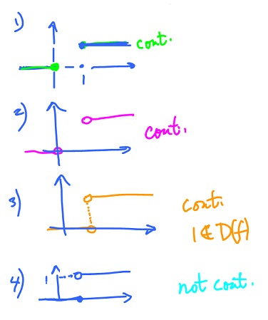
Recall, how the fact that the domain of the function is made of two pieces affects its continuity:

1. $D(f) = ( -{\infty}, 0 ] {\cup} [ 1, {\infty} )$, i.e. "two pieces" and $f$ is continuous!
2. Even if undefined at the end points, it's still continuous.
3. Even if these end points are the same point, still two pieces and still continuous. Here $1 \not\in D(f) = ( -{\infty}, 1 ) {\cup} ( 1, {\infty} )$
4. This one is not continuous! $D(f) = ( -{\infty}, 1 ] {\cup} ( 1, {\infty} ) = {\bf R}$, one piece!

(Proof of 4: Let $a = 1, x = 1 + {\epsilon}, {\epsilon} > 0. | f(x) - f(a) | = | 1 - 0 | = 1.$ Finish...)

What is the point? Continuity of a function depends on the topology of its domain, specifically, its connectedness.

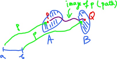
Suppose $X = A {\cup} B {\subset} {\bf R}^n$ and $A$ and $B$ are disjoint.

Is there a continuous path from $P$ to $Q$?

If yes, $X$ is connected, if no, then disconnected.

Definition. A subset $X$ of ${\bf R}^n$ is called path-connected if for any $P, Q {\in} X$ there is a continuous function $p: [ a, b ] {\rightarrow} {\bf R}^n$ such that

$$p(a) = P, p(b) = Q.$$

Examples:

Theorem. $X = {\bf R}^n$ is path-connected.

Proof. In order to prove the claim, we have to find the path from $P$ to $Q$ for any given $P, Q {\in} {\bf R}^n$. The idea is to use a straight line.

Define $p: [ a, b ] {\rightarrow} {\bf R}^n$ by

$$p(t) = ( Q - P ) t + P.$$

(This is a convex combination of $P$ and $Q$.) Prove now that $p$ is continuous with $p(0) = P, p(1) = Q$. QED

Exercise. Let $X = B^n$ denote a closed ball. Is it path-connected? Yes. Proof is same as above.

Exercise. Apply the same proof to show that any convex set is path-connected (think of a box, a square, a 3d cylinder, etc).

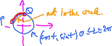
Exercise. The same proof cannot be applied for donuts or circles, since they have holes and aren't convex.

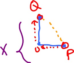
Exercise. Let $X = [ 0, 1 ] × {0} {\cup} {0} × [ 0, 1 ],$ where

$[ 0, 1 ] \times \{0 \}$ denotes the horizontal axis and is path-connected,
$[ 0, 1 ] \times \{0 \}$ denotes the vertical axis and is path-connected.

Let further $P = ( 1, 0 ), Q = ( 0, 1 ).$

Now let us find the path from $P$ to $Q$. Define piecewise

$p(t) = ( 1 - t, 0 ), u \leq t \leq 1$ (continuous), and
$p(t) = ( 0, t - 1 ), 1 \leq t \leq 2$ (continuous).

In order to prove continuity, we verify only at point $a = 1$. Finally, $p: [ 0, 2 ] {\rightarrow} {\bf R}^2$ "Image",

$p(0) = ( 1 - 0, 0 ) = ( 1, 0 ) = P,$
$p(2) = ( 0, 2 - 1 ) = ( 0, 1 ) = Q.$

Theorem. If $A, B$ are path-connected and $A \cap B \neq \emptyset$, then $A {\cup} B$ is path-connected.

Proof The idea is to combine functions for $A$ and $B$. Given $P, Q {\in} A {\cup} B$, find the path. Pick $N {\in} A \cap B$. Suppose $P {\in} A, Q {\in} B$. From connectedness of $A$ and $B$ it follows that we can

• find the path from $P$ to $N$, where $p: [ a, b ] {\rightarrow} A$, and
• find the path from $N$ to $Q$, where $q: [ c, d ] {\rightarrow} B$.

Then combine $p$ and $q$ into a path from $P$ to $Q$. Define

$r(t) =$ piecewise... (how?)

with $r$ continuous, $r: [ \cdot ] {\rightarrow} {\bf R}^n$. QED

Exercise. Let $X$ be a circle, which is not convex. Prove that $X$ is connected. Give an explicit formula for the path.

Theorem (Path-connectedness in ${\bf R}$). In ${\bf R}$, the path-connected sets are:

• intervals (open, closed, half-open, finite, infinite),
• single points,
• the empty set,

and these only

In order to prove the theorem, show

1. These sets are connected, i.e., construct a continuous function on an interval (they are convex!).
2. There are no other connected sets.

Theorem. The image of a path-connected set under a continuous function is path-connected, or: $f: {\bf R}^n {\rightarrow} {\bf R}$ continuous and $A {\subset} {\bf R}^n$ is path-connected, then

$f(A)$ is path-connected.

Recall from Calc1.

Intermediate Value Theorem. Let $A = f(a), B = f(b)$, and $f$ continuous.

Let further $A \leq C \leq B.$ Then there is $c {\in} [ a, b ]$ with $f(c) = C$.

Observe that if $A, B {\in} f( [ a, b ])$, then $C {\in} f( [ a, b ])$. What does it tell about the topology of $f( [ a, b ])$?

Rephrased IVT. $f( [ a, b ])$ is path-connected (an interval).

Then more general is this.

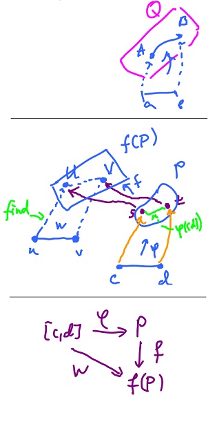
Theorem. Let $f: {\bf R}^n {\rightarrow} {\bf R}^m$ and $P {\subset} D(f) {\subset} {\bf R}^n$ be path-connected. Then $f(P)$ is path-connected.

Proof. Idea: re-state the problem of finding the necessary path in $f(P)$ as a problem of finding a certain path in $P$.

Recall the definition: A set $Q$ is path-connected if for any $A, B {\in} Q$ there is a continuous function $p: [ a, b ] {\rightarrow} Q$ such that

$$p(a) = A and p(b) = B.$$

Set $Q = f(P), A = V, B = V$, in this definition. We have to show that there is a continuous function

$$w: [ u, v ] {\rightarrow} f(P)$$

such that

$$w(u) = U {\rm \hspace{3pt} and \hspace{3pt}} w(v) = V.$$

Every point is $f(P)$ comes from $P$, then $U = f(s)$ and $V = f(t)$ for some $s, t {\in} P$ (preimages of $U,V$ under $f$).

We then use the path-connectedness of $P$. We set $Q = P, A = s, B = t$, in the above definition. Then there is a continuous function $\varphi: [ c, d ] {\rightarrow} P$ such that $\varphi(c) = s, \varphi(d) = t.$

Now let $w = f {\circ} \varphi$, and let $u = c, v = d.$

Then

1. $w$ is continuous as the composition of two continuous functions (above),
2. $w(u) = f ( \varphi(u) ) = f( \varphi(c) ) = f(s) = U, w(v) = f ( \varphi(v) ) = f( \varphi(d) ) = f(t) = V.$

Then function $p = w$ satisfies the above definition. QED

Limit points

Recall from Calc 1. Consider a sequence $A = \{ \frac{1}{n}: n = 1, 2, ... \} {\subset} {\bf R}.$ Then

$$\displaystyle\lim_{n \rightarrow \infty} \frac{1}{n} = 0,$$

i.e. $0$ is the limit of the sequence $A$. Here we take a slightly different approach. Here we ignore the order of points in $A$ and say $0$ is a limit point of the set $A$.

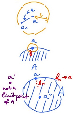
Definition. Given a subset of $A$ of ${\bf R}^n$, the point $a {\in} {\bf R}^n$ is called a limit point of $A$ if every open ball $B( a, {\epsilon} )$ contains at least one point of $A$ other than $a$.

This is the goal. Recall that

$\displaystyle\lim_{n \rightarrow \infty} \frac{1}{n} = 0$, or
$\frac{1}{n} {\rightarrow} 0$ as $n {\rightarrow} {\infty}$,

means that $\frac{1}{n}$ is getting closer and closer to $0$. More precisely:

Definition. Suppose $a_n$ is a sequence in ${\bf R}$. We say $a_n$ converges to $a$ or $a$ is the limit of $a_n$,

$$a_n {\rightarrow} a$$

if for $n > N$ it follows that $| a_n - a | < {\epsilon}$ for $a_n {\in} {\bf R}$.

In ${\bf R}^m$, we simply replace $|\cdot|$ with $||\cdot||$ in the last line:

$|| a_n - a || < {\epsilon}$ for $a_n {\in} {\bf R}^m.$

Example. Let $a_n = a$, then $a_n {\rightarrow} a$ as $| a_n - a | = 0$.

Recall more results from Calc 1.

Theorem. Any bounded sequence has a convergent subsequence.

Theorem. A bounded monotone sequence (in ${\bf R}$) converges.

Restate the definition: $a_n {\rightarrow} a$ if for any ${\epsilon} > 0$ there is $N$ such that for $n > N, a_n {\in} B( a, {\epsilon} )$.

One more time: point $a$ is a limit point of $A$ if for any ${\epsilon} > 0$ there is $b {\in} B( a, {\epsilon} )$ with $b {\in} A$ and $b \neq a$.

Or:

$$b_n {\rightarrow} a {\rm \hspace{3pt} with \hspace{3pt}} b {\in} A {\rm \hspace{3pt} and \hspace{3pt}} b_n \neq a.$$

Exercise. Let $A = { a }.$ Is $a$ a limit point of $A$? No.

Exercise. Let $A = \{ 0 \} {\cup} ( 1, 2 ) {\subset} {\bf R}.$ Then the set of limit points of A is $[ 1, 2 ]$.

Exercise. Let $A = \{ \frac{1}{n}: n = 1, 2, ... \}.$ Then the only limit point of $A$ is $0$.

Limit of function

We concentrate on limits of functions at the limit points of their domains.

Example. Consider $f(x) = x$ for $x \neq 1$ with $D(f) = ( -{\infty}, 1 ) {\cup} ( 1, {\infty} ).$

Even though the function is undefined at $1$, the limit

$$\displaystyle\lim_{x \rightarrow 1} f(x)$$

makes sense, because $1$ is a limit point of $D(f)$.

Example. Let $f(x) = 1, D(f) = { 0 } {\cup} [ 0, 2 ).$ Here the limit

$$\displaystyle\lim_{x \rightarrow 0} f(x)$$

does not make sense.

Example. Also, if $D(f) = ( 1, {\infty} ),$ then the limit

$$\displaystyle\lim_{x \rightarrow \infty} f(x)$$

does make sense.

Definition. Suppose $f: {\bf R}^n {\rightarrow} {\bf R}$ and $a$ a limit point of $D(f)$. Then $L {\in} {\bf R}$ is the limit of $f$ as $x {\rightarrow} a$ if

for any ${\epsilon} > 0$ there is a ${\delta} > 0$ such that $|| x - a || < {\delta}$ with $x {\in} D(f) \rightarrow | f(x) - L | < {\epsilon}$.

Note 1: there is always such an $x$ - on the right - for any ${\delta} > 0$.)

Note 2: if $f: {\bf R}^n {\rightarrow} {\bf R}^m$, then $L {\in} {\bf R}^m$ and we replace in the definition the absolute value $| \cdot |$ with the norm $|| \cdot ||$ , as before:

$$|| x - a || < {\delta} {\rm \hspace{3pt} with \hspace{3pt}} x {\in} D(f) \rightarrow | f(x) - L | < {\epsilon}.$$

Note 3: Is the limit well-defined?

Theorem (Uniqueness of Limit). If $L$ and $M$ satisfy the definition, then $L = M$.

Proof'.' Let $L \neq M, L, M {\in} {\bf R}$. Say $L > M$, then let

$${\epsilon} = \frac{L - M}{2}.$$

Apply the definition with this ${\epsilon}$. Then there is a ${\delta}$ satisfying the condition. Now choose $x {\in} D(f)$ with

$$|| x - a || < {\delta}.$$

Then it follows that $| f(x) - L | < {\epsilon}, | f(x) - M | < {\epsilon}.$

(Provide the details here!)

Then

$$| f(x) - L | + | f(x) - M | < 2{\epsilon} = L - M.$$

Finish the proof. QED

Theorem. Let $\displaystyle\lim_{x \rightarrow a} f(x) = L, \displaystyle\lim_{x \rightarrow a} g(x) = M.$ Then

1. $\displaystyle\lim_{x \rightarrow a} ( f(x) + g(x) ) = L + M$,
2. $\displaystyle\lim_{x \rightarrow a} ( f(x) ⋅ g(x) ) = L ⋅ M$,
3. $\displaystyle\lim_{x \rightarrow a} ( f(x) / g(x) ) = L / M$, provided $M \neq 0$.

Theorem (Limits Under Composition). For the two cases

1. $f: {\bf R} {\rightarrow} {\bf R}^n, g: {\bf R}^n {\rightarrow} {\bf R}$,
2. $f: {\bf R}^n {\rightarrow} {\bf R}, g: {\bf R} {\rightarrow} {\bf R}^n$

let $\displaystyle\lim_{x \rightarrow a} f(x) = L, \displaystyle\lim_{t \rightarrow L} g(t) = M.$

Then $\displaystyle\lim_{x \rightarrow a} ( g \circ f )(x) = M.$

Theorem. The function $f$ is continuous at $x = a$ iff

$$\displaystyle\lim_{x \rightarrow a} f(x) = f(a).$$

The point $a$ is a limit point of $D(f)$.

Example. Let $f( x, y ) = x + y$ continuous on $D(f)$,

$$D(f) = { ( x, 0 ): x {\in} {\bf R} } {\subset} {\bf R}^2.$$

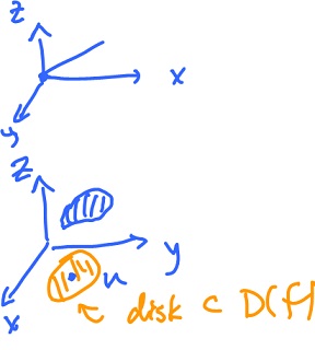
Consider points in $D(f)$ that have a ball around them that lies entirely in $D(f)$, interior point $D(f)$. (This is unlike the first example.)

Definition. Given $A {\subset} {\bf R}^n$, the point $a {\in} A$ is called an interior point of $A$ if there is an ${\epsilon} > 0$ such that

$$B( a, {\epsilon} ) {\subset} A.$$

Let $n = 1$. Is a an interior point of $A = \{ a \}$? No.

$A = [ 0, 1 ]$. What are the interior points? All but $0$ and $1$.

The set of all interior points of $A$ is called the interior of $A$, and we write ${\rm int \hspace{3pt}} A$.

The interior

$${\rm int \hspace{3pt}}[ 0, 1 ] = ( 0, 1 ),$$

as the limit points of $[ 0, 1 ]$ are $[ 0, 1 ]$, so $0$ and $1$ are limit points but not interior points.

Is vice versa possible? No. Every interior point is a limit point (see Theorem).

Consider $B( a, r ) = \{ x {\in} {\bf R}^n: | x - a | \leq r \}$, a closed ball, then

$${\rm int \hspace{3pt}} B( a, r ) = \{ x {\in} {\bf R}^n: | x - a | < r \},$$

i.e. an open ball.

For more see Limit of function.

Directional derivatives

When computing a limit, like

$$\displaystyle\lim_{x \rightarrow a}f(x),$$

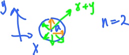
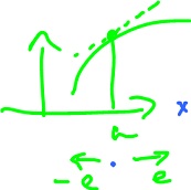
in dimension $1$, point $a$ is "approached" by $x$. It can happen in a number of ways but from two directions only: left and right. In dimension $n$, there are infinitely many possible directions and $x$ can approach from any of them - if $a$ is an interior point of $D(f)$.

Let $n = 2, z = f( x, y ).$

Then there are two main cases of how $z$ can approach some $a$:

1. $z$ depends on $x$ only,
2. $z$ depends on $y$ only.

These two cases lead to the concept of partial derivatives.

Let $n = 1, y = f(x),$ then the derivative is the rate of change of $y$ with respect to $x$. We will use this concept initially to study the rates of change (corresponding to many possible directions) of functions of several variables.

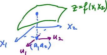
We start with dimension $2$. In this low dimension, we can still visualize the function. In particular, the output $z$ can be treated as the altitude of a surface at the point $( x, y )$ on the plane.

Problem. Find the rate of change of $z$ as we move in a given direction to and from point $a$.

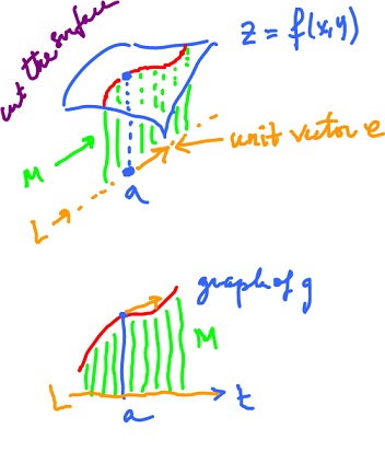
We approach the problem by creating a new function - a function of one variable. How? Take the graph

$$z = f(u), z {\in} {\bf R}, n {\in} {\bf R}^n, a {\in} {\bf R}^n.$$

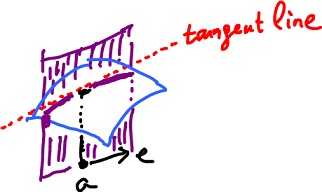
Now choose a direction, a unit vector $e {\in} {\bf R}^n$ that follows the given direction. The point $a$ and the vector $e$ together define a line (a $1$-dimensional affine subspace) $L$:

$$u = a + te, t {\in} {\bf R}.$$

Consider

$$M = \{ ( u, z ): z {\in} {\bf R}, u {\in} L \} {\subset} {\bf R}^{n+1}.$$

$M$ is a plane, an affine subspace. Consider the intersection of the graph of $f$ and the plane $M$, the result is a curve (if $f$ is continuous). We will deal with a restriction of $f$ to $L, D(g) = L$. Now every element $v$ in $L$ has the form

$$u = a + te.$$

Define

$$g(t) = f( a + te ).$$

This is a function of one variable, $t$. Then $g'(t)$ is

$$g'(0) = \displaystyle\lim_{h \rightarrow 0} \frac{g( 0 + h ) - g(0)}{h},$$

which is the slope of the tangent line to the curve at this point.

Example. Let $f( x, y ) = x y, a = ( 1, 0 ), e = ( \frac{1}{\sqrt{2}}, \frac{1}{\sqrt{2}} )$, further

$$L = \left\{ ( 1, 0 ) + t \left( \frac{1}{\sqrt{2}}, \frac{1}{\sqrt{2}} \right): t {\in} {\bf R} \right\},$$

$$\begin{array}{} g(t) &= f \left( ( 1, 0 ) + t \left( \frac{1}{\sqrt{2}}, \frac{1}{\sqrt{2}} \right) \right) &= f \left( 1 + \frac{t}{\sqrt{2}}, 0 + \frac{t}{\sqrt{2}} \right) &= \left( 1 + \frac{t}{\sqrt{2}}) \cdot ( \frac{t}{\sqrt{2}} \right)^2 &= \left( 1 + \frac{t}{\sqrt{2}} \right) \cdot \frac{t^2}{2} &= \frac{t^2}{2} + \frac{t^3}{2\sqrt{2}}, \end{array}$$

$$g'(t) = t + \frac{3}{2 \sqrt{2}} t^2,$$

and

$$g'(0) = 0.$$

Definition. The directional derivative of $z = f(u)$ at $u = a$ in the direction of a unit vector $e$ is

$${\nabla}_e f(a) = \displaystyle\lim_{h \rightarrow 0} \frac{f( a + he ) - f(a)}{h}.$$

Note 1: $\frac{f( a + he ) - f(a)}{h}$ is a scalar function of $h$ from ${\bf R} {\rightarrow} {\bf R}$.

Note 2: if $k = -h$, then

$$\displaystyle\lim_{k \rightarrow 0} \frac{f( a + ke ) - f(a)}{-k} = - {\nabla}_e f(a).$$

So ${\nabla}_e f(a) = -{\nabla}_{-e} f(a)$. Indeed, consider an example in dimension $1$:

$${\nabla}_{-1} x^2 |_{x=1} = \displaystyle\lim_{h \rightarrow 0} \frac{( 1 + h(-1) )^2 - 1^2}{h}$$

and

$$( x^2 )' |_{x=1} = {\nabla}_1 x^2 |_{x=1} = \displaystyle\lim_{h \rightarrow 0} \frac{( 1 + h - 1 )^2 - 1^2}{h}.$$

Example. $$\begin{array}{} \displaystyle\lim_{h \rightarrow 0} \frac{1}{h} ( f( ( 1, 0 ) + h ( \frac{1}{\sqrt{2}}, \frac{1}{\sqrt{2}} ) ) - f( 1, 0 ) ) &= \displaystyle\lim_{h \rightarrow 0} \frac{1}{h} ( f( ( 1 + \frac{h}{\sqrt{2}}, \frac{h}{\sqrt{2}} ) ) - f( 1, 0 ) ) \\ &= \displaystyle\lim_{h \rightarrow 0} \frac{1}{h} ( ( 1 + \frac{h}{\sqrt{2}} )( \frac{h}{\sqrt{2}} )^2 ) - 0 ) \\ &= \displaystyle\lim_{h \rightarrow 0} ( 1 + \frac{h}{\sqrt{2}} ) \frac{h}{2} \\ &= 0. \end{array}$$

Example. Consider $f( x_1, x_2 ) = 1 - 2x_1 + 3x_2$ at $a = ( 2, -1 )$. Find the directional derivative "in the direction" of $v = ( 3, 4 )$.

You can't use $u$ as the direction as the direction has to be a unit vector. So, find $e$ first:

$$e = \frac{v}{|| v ||} = - \frac{( 3, 4 )}{( 3^2 + 4^2 )^{\frac{1}{2}}} = ( 3 / 5, 4 / 5 ).$$

Finish.

For more see Directional derivative.

Partial derivatives

${\bf R}^n$: Given $z = f(u)$ at $u = a$, then $$\begin{array}{} \frac{\partial f}{\partial x_1} (a) = {\nabla}_e f(a) {\rm \hspace{3pt} for \hspace{3pt}} e = ( 1, 0, ..., 0 ), \\ \vdots \\ \frac{\partial f}{\partial x_n} (a) = {\nabla}_e f(a) {\rm \hspace{3pt} for \hspace{3pt}} e = ( 0, 0, ..., 1 ). \end{array}$$

Partial derivatives are particular cases of directional derivatives.

$$f' = \left( \frac{\partial f}{\partial x_1}, ..., \frac{\partial f}{\partial x_n} \right)$$

the gradient.

As it turns our we can turn this around and recover all directional derivatives.

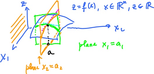
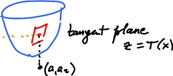
Consider $z = f(x), x {\in} {\bf R}^n, z {\in} {\bf R}, x = ( x_1 x_2 ), a = ( a_1 a_2 ).$

1. Cut the graph of $f$ with a plane parallel to the $x_1,z$-plane. The result is a curve $z = f ( x_1, a_2 ),$ and the slope of the tangent line is $\frac{\partial f}{\partial x_1}(a)$, which is the derivative of $z = f ( \cdot, a_2 ).$
2. Cut the graph of $f$ with a plane parallel to the $x_2,z$-plane. The result is a curve $z = f ( a_1, x_2 ),$ and the slope of the tangent line is $\frac{\partial f}{\partial x_n}(a).$

Let's compare to the directional derivative? The picture is very similar. The plane is spanned by $e$ and $( 0, 0, 1 )$. Cut a curve from the graph. Then

$${\nabla}_e f(a)$$

is the slope of the curve at $x = a$.

Higher order partial derivatives are the derivatives of the partial derivatives:

$$\frac{\partial f}{\partial x_1}, ..., \frac{\partial f}{\partial x_n}$$

are functions from ${\bf R}^n {\rightarrow} {\bf R}$ and can also be differentiated with respect to $x_1, ..., x_n$ each.

From

$$\frac{\partial f}{\partial x_1}$$

we get $n$ second derivatives

$$\frac{\partial}{\partial x_k} \left( \frac{\partial f}{\partial x_1} \right)$$

and so on. Altogether, we have $n^2$ second derivatives.

Frequently it's less though.

Example. Let $f( x, y ) = x^2 y$.

Then

$$\frac{\partial f}{\partial x} = 2xy, \frac{\partial f}{\partial y} = x^2,$$

$$\frac{\partial}{\partial y} ( \frac{\partial f}{\partial x} ) = 2x, \frac{\partial}{\partial x} ( \frac{\partial f}{\partial y} ) = 2x.$$

Same!

These two are called mixed second derivatives.

The meaning of the others is clear. For example, $\frac{\partial^2f}{\partial x^2}$ is the concavity of $z = f( x, a_2 )$.

Analogously for $\frac{\partial^2 f}{\partial y^2}$.

Other notation for these is:

• $\frac{\partial^2 f}{\partial x \partial y}$
• $\frac{\partial^2 f}{\partial x_1 \partial x_2}$
• $\frac{\partial^2 f}{\partial x_1^2}$
• $D_{1234}f$
• $f_{xy}$
• $f_{xx}$

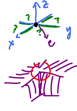
Example. It is possible that $\frac{\partial f}{\partial x}$ and $\frac{\partial f}{\partial y}$ exist, but some directional derivatives do not.

Consider the graph $z = f( x, y )$ with $f( 0, y ) = f( x, 0 ) = 0.$ Then

$$\frac{\partial f}{\partial x} = \frac{\partial f}{\partial y} = 0 {\rm \hspace{3pt} at \hspace{3pt}} ( 0, 0 ),$$

and ${\nabla}_e f$ might not exist at $0$ because of the vertical drop. Specifically,

$$f( x, y ) = \frac{2xy^2}{x^2 + y^2} {\rm \hspace{3pt} if \hspace{3pt}} ( x, y ) \neq 0, $$

$$f( x, y ) = 0 {\rm \hspace{3pt} if \hspace{3pt}} ( x, y ) = 0.$$

For more see Partial derivatives.

Approximations

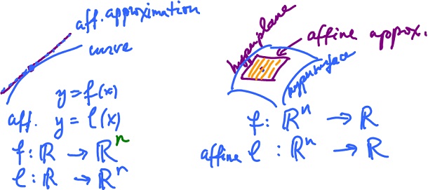
Consider the idea of "linear approximation", or more precisely, "affine approximation", in dimension $1$ and then see how it translates into dimension $2$.

As the picture shows, a curve is approximated by a straight line while a surface by a plane.

• Dim $1$: given a function $f: {\bf R} {\rightarrow} {\bf R}$, an affine function $l: {\bf R} {\rightarrow} {\bf R}$ is its approximation.
• Dim $n$ parametric curve: given a function $f: {\bf R} {\rightarrow} {\bf R}^n$, an affine function $l: {\bf R} {\rightarrow} {\bf R}^n$ is its approximation.
• Dim $n$ function of several variables: given a function $f: {\bf R}^n {\rightarrow} {\bf R}$,

graph ${\subset} {\bf R}^n \times {\bf R} = {\bf R}^{n+1}$, an affine function $l: {\bf R}^n {\rightarrow} {\bf R}$,

The last item is a plane in dimension $2$, or a hyperplane in ${\bf R}^n \times {\bf R}$.

The idea comes from the fact that if you zoom in on the graph of a differentiable function, it looks like a straight line.

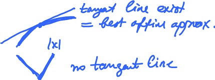
Example. Let $f(x) = | x |$. Then

$${\nabla}_1 f(0) = 1,$$

$${\nabla}_{-1} f(0) = 1,$$

i.e. they are not aligned! Hence $f'(0)$ does not exist as there is no affine approximation.

Recall, an affine function $L: {\bf R}^n {\rightarrow} {\bf R}^m$ (graph is a hyperplane) can be written as

$$L(x) = u_0 + A(x),$$

where $u_0 {\in} {\bf R}^m, x {\in} {\bf R}^n$, and $A: {\bf R}^n {\rightarrow} {\bf R}^m$ linear. $A$ is a matrix $A(x) = Ax$ of dimension $m \times n$.

Example. Consider the above case with $m = 1$. Then

$$L(x) = u_0 + A(x), $$

where $A$ is of dimension $1 \times n$ and $x$ is of dimension $n \times 1, u {\in} {\bf R}$ a number, $x {\in} {\bf R}^n$. In this special case, $A$ is a vector and

$$Ax = A \cdot x {\rm \hspace{3pt} (inner \hspace{3pt} product)}.$$

Example. Consider the above case with $m = 3$. Let further $A = ( 1, 2, 3 )$ be a linear map, $u_0 = 5$. Then

$$\begin{array}{} L(x) &= 5 + ( 1, 2, 3 ) \cdot ( x_1, x_2, x_3 ) \\ &= 5 + x_1 + 2x_2 + 3x_3 \end{array}$$

a hyperplane.

Definition. Let $f: {\bf R}^n {\rightarrow} {\bf R}^m$, $a$ an interior point of $D(f)$. The best affine approximation $T: {\bf R}^n {\rightarrow} {\bf R}^m$ is an affine function satisfying the conditions:

1. $f(a) = T(a)$;
2. $\displaystyle\lim_{x \rightarrow a} \frac{f(x) - T(x)}{|| x - a ||} = 0$.

Note 1: The best affine approximation is well defined. Why?

Note 2: Let $\displaystyle\lim_{x \rightarrow a} ( f(x) - T(x) ) = 0.$ Then $f(x) - T(x) = 0$ if $f$ and $T$ are continuous, hence

$$f(a) = T(a) {\rightarrow} (1).$$

Let $f: {\bf R}^n {\rightarrow} {\bf R}^m$. What is the form of $T$?

$$T(x) = z + L( x - a ),$$

where $z$ is constant and $L$ is linear. Further,

$$\begin{array}{} f(a) &= T(a) {\rm \hspace{3pt} (by \hspace{3pt} (1) \hspace{3pt} )} \\ &= z + L( a - a ) \\ &= z + L(0) \\ &= z, \end{array}$$

so $T(x) = f(a) + L( x - a )$ for each $a$,

or $T(x) = f(a) + L_a( x - a )$ for each $a$,

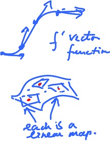
where the first term is constant and the second is a linear map evaluated at $x-a$. This linear map $L_a$ is called the total derivative of $f$ at $x = a$.

Example. Let $f( x_1, x_2 ) = x_1^2 + x_2^2$ and $a = ( 1, 2 )$. The graph is a paraboloid. Check that

$$T(x) = T( x_1, x_2 ) = 5 + 2 ( x_1 - 1 ) + 4 ( x_2 - 2 )$$

is the best affine approximation. By definition:

(1)$$\begin{array}{} T(a) &= T( 1, 2 ) \\ &= 5 + 2 ( x_1 - 1 ) + 4 ( x_2 - 2 ) \\ &= 5 + 2 ( 1 - 1 ) + 4 ( 2 - 2 ) = 5 + 0 + 0 \\ &= 5 \\ &= f( 1, 2 ) {\rm \hspace{3pt} as} \\ f( 1, 2 ) &= 1^2 + 2^2 = 5, \end{array}$$

(2) $$\frac{f(x) - T(x)}{| x - a |} = ( ( x_1^2 + x_2^2 ) - \frac{5 + 2 ( x_1 - 1 ) + 4 ( x_2 - 2)}{( x_1 - 1 )^2 + ( x_2 - 2 )^2 )^{\frac{1}{2}}},$$

where the denominator approaches $0$ as $x {\rightarrow} a$.

Then, canceling the denominator, we obtain $$\begin{array}{} \frac{f(x) - T(x)}{| x - a |} &= \frac{( x_1 - 1 )^2 + 2x_1 - 1 + ( x_2 - 2 )^2 ) + 4x_2 - 4) - 5 + 2( x_1 - 1 ) + 4 ( x_2 - 2 )}{\sqrt{}..} \\ &= \frac{( x_1 - 1 )^2 + 2x_1 - 1 + ( x_2 - 2 )^2 + 4x_2 - 4 - 5 + 2 - 4x_2 + 5}{\sqrt{}..} \\ &= \frac{( x_1 - 1 )^2 + ( x_2 - 2 )^2}{( ( x_1 - 1 )^2 + ( x_2 - 2 )^2 )^{\frac{1}{2}}} \\ &= ( ( x_1 - 1 )^2 + ( x_2 - 2 )^2 )^{\frac{1}{2}} {\rightarrow} 0 {\rm \hspace{3pt} as \hspace{3pt}} x_1 {\rightarrow} 1, x_2 {\rightarrow} 2. \end{array}$$

So, $T(x) = 5 + 2 ( x_1 - 1 ) + 4 ( x_2 - 2 )$ is the best affine approximation of $f( x_1, x_2 ) = x_1^2 + x_2^2$ around $a = ( 1, 2 )$.

Then, the total derivative

$$L_a( x - a ) = L_{(1,2)} ( x_1 - 1, x_2 - 2 ) = 2 ( x_1 - 1 ) + 4 ( x_2 - 2 ).$$

Hence, $L_{(1,2)}( u_1, u_2 ) = 2u_1 + 4u_2$ is the total derivative.

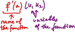
Notation: We write

• $f'(a)$ for $L_a$,
• $f'(a)( u_1, u_2 )$ for $L_{(1,2)}( u_1, u_2 )$, where $u_1, u_2$ are variables of $L_a$.

Note that $f'(a)( u_1, u_2 )$ is linear with respect to $u_1, u_2$, not to $a$, and $f'(a)$ is the name of the function, $u_1, u_2$ are the variables of the function.

Further,

$$u_1 = x_1 - 1,$$

$$u_2 = x_2 - 2.$$

Then with $f( x_1, x_2 ) = x_1^2 + x_2^2$, we obtain

$$\frac{\partial f}{\partial x_1}|_{(1,2)} ( x_1, x_2 ) = 2x_1 |_{(1,2)} = 2 \cdot 1 = 2,$$

$$\frac{\partial f}{\partial x_2}|_{(1,2)} ( x_1, x_2 ) = 2x_2 |_{(1,2)} = 2 \cdot 2 = 4.$$

With partial derivatives equal to $2$ and $4$, we obtain

$$\begin{array}{} f'( 1, 2) ( u_1, u_2 ) &= 2u_1 + 4u_2 &= ( 2, 4 ) \cdot ( u_1 , u_2 ) &= {\nabla}f( 1, 2 ) \cdot ( u_1 , u_2 ) {\rm \hspace{3pt} (as \hspace{3pt}} {\nabla}f( 1, 2 ) = ( 2, 4 )) \end{array}$$

which is linear $(f'( 1, 2)$ is a linear map).

Claim:

$$f'(a)(u) = {\nabla}f(a) \cdot u,$$

i.e. a computational formula for the total derivative.

Note that $f'(a)(u)$ is defined via properties (1) and (2), and ${\nabla}f(a)$ is the gradient.

Here we have a function

$$z = f(x), x {\in} {\bf R}^n, z {\in} {\bf R},$$

its partial derivatives are computed and interpreted as tangent lines to the graph of $f$, within the corresponding vertical planes. Finally, these two lines span a plane, called the tangent plane.

Theorem. Suppose $a$ is an interior point of $D(f)$ with $f: {\bf R}^n {\rightarrow} {\bf R}$. Further suppose partial derivatives $\frac{\partial f}{\partial x_k}$ exist and are continuous on an open ball centered at $a$. Then $f'(a)$ exists, i.e. $f$ is differentiable.

So, if the tangent line exists, it is the best affine approximation. Or no tangent line exists,

Example. Let $f( x, y ) = x^2.$ Consider $g(x) = x^2$.

What is the relation between $f'( x, y )$ and $g'(x)$?

$$\frac{\partial f}{\partial x} = g'(x),$$

$$\frac{\partial f}{\partial y} = 0.$$

For more see Affine approximation.