Classes of functions

The simplest functions

In this chapter, we will study some specific functions as well as some broad categories of functions. We start with the former.

In the most general situation, there are always two functions that are very simple.

Let's consider the two sets we considered in Chapter 2:

• $X$ is the five boys and
• $Y$ is the four balls.

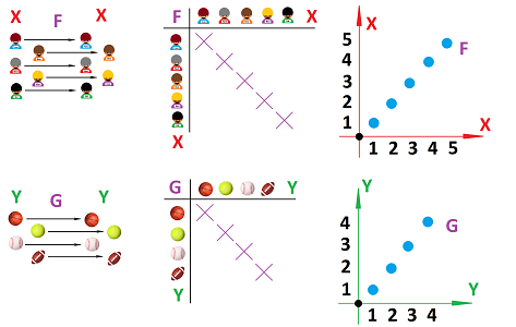
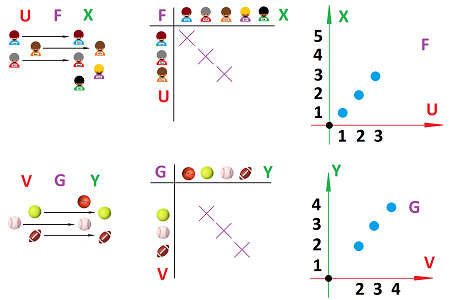
Now, what if all boys prefer basketball? Then the “preference function” $F$ cannot be simpler: all of its values are equal and all arrows point at the basketball.

The table of this function $F$ is also very simple: all crosses are in the same column; and the graph has all dots on the same horizontal line. The value of $y=F(x)$ doesn't vary as $x$ varies; it is constant.

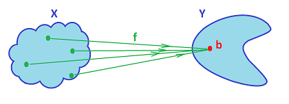
Definition. Suppose sets $X$ and $Y$ are given. A function $f:X\to Y$ is a constant function, i.e., for some specified element $b$ of $Y$, we set: $$f(x)=b,\ \text{ for all } x.$$

In the generic illustration below, all arrows converge on one output:

The graph of a constant numerical function is a horizontal line:

Of course, if the domain is disconnected, then so is the graph.

Example. Constant functions are convenient building blocks for more complex functions. This is a familiar example of how we build from three constant functions a single “piece-wise constant” function: $$\begin{array}{ccc} y=\operatorname{sign}(x):& x & \mapsto & \begin{array}{|c|}\hline &x& \begin{array}{lllll} \nearrow_{\text{ if }x> 0} &\begin{array}{|c|}\hline\quad \text{ choose }1 \quad \\ \hline\end{array} & \mapsto & y & \searrow\\ \to_{\text{ if }x=0} &\begin{array}{|c|}\hline\quad \text{ choose }0 \quad \\ \hline\end{array} & \mapsto & y & \to\\ \searrow_{\text{ if }x<0} &\begin{array}{|c|}\hline\quad \text{ choose }-1 \quad \\ \hline\end{array} & \mapsto & y & \nearrow\\ \end{array}& y\\ \hline\end{array} & \mapsto & y \end{array}.$$ If there many different values and we zoom out from the graph of such a function, it might look like a curve:

$\square$

Exercise. Build a few such functions from sequences following Chapter 1.

What can we say about compositions of this special function, $f$, with another, $g$? Consider this diagram: $$\newcommand{\ra}[1]{\!\!\!\!\!\xrightarrow{\quad#1\quad}\!\!\!\!\!} \newcommand{\da}[1]{\left\downarrow{\scriptstyle#1}\vphantom{\displaystyle\int_0^1}\right.} \begin{array}{ccc} X& \ra{ f }& Y & \ra{ g }& Z\\ \hline x_1&&y_1&\to&z_1\\ &\searrow&&&\\ x_2&\to&y_2&\to&z_2\\ &\nearrow&&&&\\ x_3&&y_3&\to&z_3.\\ \end{array}$$ The output is the same for all $x$! And here is another one: $$\newcommand{\ra}[1]{\!\!\!\!\!\xrightarrow{\quad#1\quad}\!\!\!\!\!} \newcommand{\da}[1]{\left\downarrow{\scriptstyle#1}\vphantom{\displaystyle\int_0^1}\right.} \begin{array}{ccc} Z& \ra{ g }& X & \ra{ f }& Y\\ \hline z_1&\to&x_1&&y_1\\ &&&\searrow\\ z_2&\to&x_2&\to&y_2\\ &&&\nearrow\\ z_3&\to&x_3&&y_3.\\ \end{array}$$ Again, the output is the same for all $y$! I So, whether the other function comes after (case 1) or before (case 2) a constant function, the result is the same; this is our conclusion.

THEOREM. The composition of any function with a constant function is a constant function.

Proof. This is the algebra for case 1: $$x\mapsto f(x)=b\ \Longrightarrow\ x\mapsto g(f(x))=g(b).$$ This is the algebra for case 2: $$y\mapsto g(y)=x \ \Longrightarrow\ y\mapsto f(g(y))=b.$$ $\blacksquare$

As a transformation of the line, the constant function is extreme; it “crushes” (or collapses) the whole line into a single point:

At the other end of the spectrum is another extreme transformation; it “does nothing” to the line:

So, for our set $X$ of boys, we have a special function $G$ from $X$ to $X$ (and another from $Y$ to $Y$ for the balls). Each arrow comes back to the boy (or ball) it started with:

The table of this function $G$ is also very simple: all crosses are on the diagonal; and the graph has all dots on the diagonal. The output of $G$ is identical to the input.

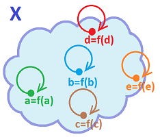
Definition. Suppose one set $X$ is given. The identity function $I:X\to X$ is given by: $$I(x)=x,\ \text{ for all } x.$$

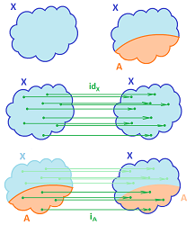
In the generic illustration below, every arrow circles back to its input:

What can we say about compositions of this special function, $I$, with another, $g$? Whether the other function comes before or after the identity function, the result is the same; this is our conclusion.

THEOREM. A composition of any function with the identity function is that function: $$I\circ g=g,\quad g\circ I=g.$$

Proof. Consider this diagram: $$x\mapsto y=I(x)=x \ \Longrightarrow\ x\mapsto g(y)=g(I(x))=g(x).$$ The output is the same as the input! Here is the other one: $$y\mapsto x=g(y) \ \Longrightarrow\ y\mapsto I(x)=I(g(y))=g(y).$$ Again, the output is the same as the input! $\blacksquare$

A function can be represented in a number of ways; how do we know that this is the same function?

What does it mean when we say that two functions are equal? When each possible input produces the same output for the two. Suppose $f$ and $g$ are two functions, $$f:X\to Y;$$ they are equal, $f=g$, if for each $x$ in the domain, i.e., same domain for $f$ and $g$, we have $$f(x)=g(x).$$ It is illustrated in the flowchart below: $$\begin{array}{ccc} x & \mapsto & \begin{array}{c} &x& \begin{array}{lllll} \nearrow &x &\mapsto &\begin{array}{|c|}\hline\quad f \quad \\ \hline\end{array} & \mapsto & y \\ \\ \searrow &x &\mapsto &\begin{array}{|c|}\hline\quad g \quad \\ \hline\end{array} & \mapsto & u \\ \end{array} \text{same! } \end{array} \end{array}$$

Example. Consider: $$f(x)=2x+4\ \text{ and }\ g(x)=2(x+2) \ \Longrightarrow\ f=g.$$ That's what symbol manipulation is about... $\square$

What does it mean when we say that two functions are not equal? The opposite: when an input is possible that produces two different outputs for the two. Suppose $f$ and $g$ are two functions, $$f:X\to Y;$$ they are not equal, $f\ne g$, if there is $x$ -- in or out of either domain -- such that we have $$f(x)\ne g(x).$$ It is illustrated in the flowchart below: $$\begin{array}{ccc} 3 & \mapsto & \begin{array}{c} &3& \begin{array}{lllll} \nearrow &3 &\mapsto &\begin{array}{|c|}\hline\quad f \quad \\ \hline\end{array} & \mapsto & 7 &\\ \\ \searrow &3 &\mapsto &\begin{array}{|c|}\hline\quad g \quad \\ \hline\end{array} & \mapsto & 12 \\ \end{array} \text{different! } \end{array} \end{array}$$ As you can see, you only need to find a single value of $x$ for which we have a mismatch.

This case also includes the situation when the two domains are unequal: $$\begin{array}{ccc} 3 & \mapsto & \begin{array}{c} &3& \begin{array}{lllll} \nearrow &3 &\mapsto &\begin{array}{|c|}\hline\quad f \quad \\ \hline\end{array} & \mapsto & 7 &\\ \\ \searrow &3 &\mapsto &\begin{array}{|c|}\hline\quad g \quad \\ \hline\end{array} & \mapsto & \text{“not in the domain!”} \\ \end{array} \text{different! } \end{array} \end{array}$$

Example. Consider: $$f(x)=\frac{x^2}{x}\ \text{ and }\ g(x)=x \ \Longrightarrow\ f\ne g.$$ Why? Because $f$ is undefined at $x=0$ which is in the implied domain of $g$. Replacing $f$ with $g$ is an example of how not to do symbol manipulation... $\square$

An established equality of two functions is called an identity. Why? Because of the above theorem: they are connected by the identity function, $I$: $$f=g\circ I.$$

In the definition of the inverse, we take two round trips and both times we arrive where we started -- with the same final output: $$\begin{array}{ccc} \begin{array}{c} \begin{array}{lllll} \text{start}&x &\to &\begin{array}{|c|}\hline\quad f \quad \\ \hline\end{array} & \to & y \\ &||&&&&\downarrow\\ \text{finish}&x' &\leftarrow &\begin{array}{|c|}\hline\quad f^{-1} \quad \\ \hline\end{array} & \leftarrow & y \\ \end{array}& \end{array} \end{array} \qquad \begin{array}{ccc} \begin{array}{c} \begin{array}{lllll} x &\to &\begin{array}{|c|}\hline\quad f \quad \\ \hline\end{array} & \to & y &\text{finish}\\ \uparrow&&&&||&\\ x &\leftarrow &\begin{array}{|c|}\hline\quad f^{-1} \quad \\ \hline\end{array} & \leftarrow & y'&\text{start} \\ \end{array}& \end{array} \end{array}$$ We interpret this definition in terms of the identity function.

THEOREM. Two functions $f:X\to Y$ and $f^{-1}:Y\to X$ are inverses of each other if and only if these two conditions are satisfied: $$\begin{array}{|c|}\hline \quad f\circ f^{-1}=I\ \text{ and }\ f^{-1}\circ f=I. \quad \\ \hline\end{array}$$

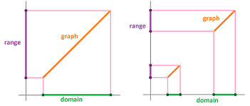
The graph of the numerical identity function is the diagonal line:

Of course, if the domain and, therefore, the codomain of this function are disconnected, then so is the graph.

The idea of such a function applies even if the two sets -- domain and codomain -- don't match. It suffices that the former is a subset of the latter. We modify the above example below:

We see $U$ included in $X$ and $V$ included in $Y$. There is only one way this can happen, and this fact creates a function.

Definition. Suppose we have a set $X$ and a subset $A$ of $X$. Then the inclusion $i: A \to X$ of $A$ into $X$ is the function defined by the following: $$i(x) = x,\ \text{ for all } x \text{ in } A.$$

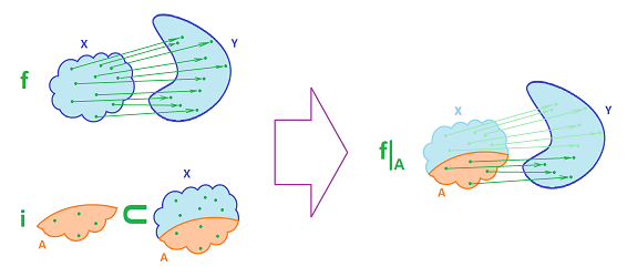
Choosing a “smaller” domain creates a new function.

Definition. Suppose we have sets $X$ and $Y$, a function $f: X \to Y$, and a subset $A$ of $X$. Then the restriction of $f$ to $A$ is a function denoted as $f\Big|_A: A \to Y$ and defined by the following: $$f\Big|_A (x) = f(x),\ \text{ for all }\ x \text{ in } A.$$

Warning: $f\Big|_A\ne f$ unless $A$ contains the domain of $f$.

Exercise. Explain how inclusions are restrictions of the identity functions.

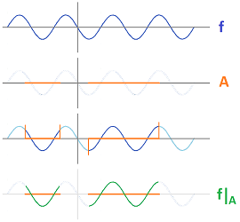
Example. Here the sine function is restricted to a subset of the real line made of two intervals.

$\square$

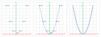
Example. Restrictions allow us to create functions that are one-to-one from those that aren't. We then build “restricted” inverses of these functions. For example, consider: $$f:{\bf R}\to {\bf R},\quad f(x)=x^2.$$ It's not invertible!

Then, we just take one, of the two, branch of the graph (no matter which one): $$g=f\Big|_{[0,+\infty)}\ \text{ or }\ g=f\Big|_{(-\infty,0]}.$$ Then, $$g:[0,+\infty) \to [0,+\infty),\quad g(x)=x^2.$$ This one is one-to-one! Its inverse is the square root: $$g^{-1}:[0,+\infty) \to [0,+\infty),\quad g^{-1}(y)=\sqrt{y}.$$ $\square$

Exercise. List all sets $A$ so that $f(x)=x^2$ restricted to $A$ is one-to-one.

Monotonicity and extreme values of functions

When an object is moving up, we also say that its altitude is increasing and then, when its falling down, the altitude is decreasing. We apply this terminology all quantities and all functions.

When we say that a function increases, we mean that the graph rises and we say it decreases when its graph drops:

This verbal definition is simple and its geometric meaning is very clear. However, both are imprecise. Even though we understand increasing functions as ones with graphs rising and decreasing functions as one with graphs falling, the precise definition has to rely on considering one pair of points at a time.

Definition. Given a function $y=f(x)$ and in interval $I$ within its domain. Then $y=f(x)$ is called increasing on interval $I$ if, for all $a,b$ in $I$, we have: $$f(a)\le f(b);$$ It is called decreasing on interval $I$ if, for all $a,b$ in $I$, we have: $$f(a)\ge f(b).$$ Together, these functions are called monotonic. The function is also called strictly increasing, strictly decreasing, and strictly monotonic, respectively, if these values cannot be equal to each other; i.e., we replace the non-strict inequality signs “$\le $” and “$\ge $” with strict “$<$” and “$>$”.

Example. Note that a constant function is both increasing and decreasing but neither strictly decreasing nor strictly increasing. $\square$

Example. An arithmetic progression is increasing when the increment is non-negative and decreasing when it's non-positive. A geometric progression is increasing when the increment is non-negative and the first element is positive. $\square$

How do we verify these conditions? Let's work out some examples algebraically.

Example. We utilize what we know about the algebra of inequalities.

First, we can multiply both sides of an inequality by a positive number: $$a<b\ \Longrightarrow\ 3a<3b.$$ Therefore, the function $f(x)=3x$ is increasing.

Second, if we multiply both sides of an inequality by a negative number, we have to reverse the sign: $$a<b\ \Longrightarrow\ (-2)a>(-2)b.$$ Therefore, the function $f(x)=-2x$ is decreasing.

Third, we can add any number to both sides of an inequality: $$a<b\ \Longrightarrow\ a+4<b+4.$$ Therefore, the function $f(x)=x+4$ is increasing. $\square$

Putting these facts together, we acquire the following.

THEOREM. A linear polynomial $$f(x)=mx+b$$

• is increasing if $m>0$, and
• is decreasing if $m<0$.

Example. This is how we can solve this problem one function at a time, from scratch. Let $$ f(x) = 3x - 7. $$ If $x_{1} < x_{2}$ then $$\begin{array}{rrclcc} f(x_{1}) = &3 x_{1} - 7 & \overset{?}{<} &f(x_{2}) = 3 x_{2} - 7 \\ \Longrightarrow &3 x_{1} & \overset{?}{<}& 3 x_{2} \\ \Longrightarrow &x_{1} & < &x_{2}. \end{array}$$ The computation suggests that $y=f(x)$ is increasing. For a complete proof, retrace these steps backwards. $\square$

Things get harder for quadratic, cubic, ... polynomials they lead to quadratic, cubic, ... inequalities.

Example. Let's consider $$f(x)=x^2.$$ First, we can multiply two inequalities, when they are aligned and their signs are positive: $$\begin{array}{ll}0<a<b\\ 0<a<b\end{array}\ \Longrightarrow\ 0<a\cdot a <b\cdot b\ \Longrightarrow\ a^2<b^2.$$ Therefore, the function $f(x)=x^2$ is increasing for $x>0$. Second, if we multiply two inequalities when their signs are negative, we have to reverse the sign: $$\begin{array}{ll}a<b<0\\ a<b<0\end{array}\ \Longrightarrow\ a\cdot a >b\cdot b>0 \ \Longrightarrow\ a^2>b^2.$$ Therefore, the function $f(x)=x^2$ is decreasing for $x<0$. $\square$

Example. Now, we let $$f(x)=x^3,$$ and follow a similar procedure starting with two unknown $a,b$ with $a<b$. We can multiply three identical inequalities -- positive or negative -- and preserve the sign: $$\begin{array}{ll}a<b\\ a<b\\ a<b\end{array}\ \Longrightarrow\ a\cdot a\cdot a <b\cdot b\cdot b\ \Longrightarrow\ a^3<b^3.$$ Therefore, the function $f(x)=x^3$ is increasing for all $x$. $\square$

Notation: We will use

• “$\nearrow$” for increasing, and
• “$\searrow$” for decreasing behavior.

In other words, we have: $$\begin{array}{l|cc} &a&<&b\\ \hline f\nearrow&f(a)& \le & f(b)\\ f\searrow &f(a) &\ge & f(b)\\ \end{array}$$

Example. In particular,

• if $f(x)=2x-3$, then $f \nearrow $ on $(-\infty, +\infty)$;
• if $g(x)=-5x+4$, then $g \searrow $ on $(-\infty, +\infty)$;
• if $h(x)=x^2$, then $h \searrow $ on $(-\infty, 0)$ and $\nearrow $ on $(0, +\infty)$;
• if $k(x)=x^3$, then $k \nearrow $ on $(-\infty, +\infty)$.

$\square$

Definition. When a function is either increasing on an interval or decreasing on it, we call it monotonic on the interval.

Example (quadratic polynomials). Things become much more complex if we need to analyze a quadratic function, $$f(x)=ax^2+bx+c,\ a\ne 0.$$ We recall that all quadratic functions are represented by parabolas (Chapter 3). They are all result of transformations of the parabola $y=x^2$. What matters especially, is the location of the vertex of the parabola: $$v=-\frac{b}{2a}.$$ The, we have:

• if $a>0$, then $f$ is strictly decreasing on $(-\infty, v)$ and strictly increasing on $(v,+\infty)$;
• if $a<0$, then $f$ is strictly increasing on $(-\infty, v)$ and strictly decreasing on $(v,+\infty)$;

For the first example, the vertex of the parabola is at $$ v = \frac{ 0 + 50 }{ 2 } = 25. $$ $\square$

THEOREM. All strictly monotonic functions are one-to-one.

Thinking geometrically, the graph of an increasing function can't come back and cross a horizontal line for the second time:

Now, algebraically, this is the definition: $$ f\nearrow \text{ when: } \underbrace{x_{1} < x_{2}}_{\text{two different inputs}} \Longrightarrow \underbrace{f(x_{1}) < f(x_{2})}_{\text{two different outputs}} .$$ Hence $f$ is one-to-one.

What about the converse, are all one-to-one functions (strictly) monotonic? No, because some functions, such as sequences, might skip values:

Such a function cannot be invertible. The converse is true when the function is also “continuous”, to be discussed in Chapter 6.

THEOREM. The odd powers are one-to-one. The even powers aren't one-to-one. The even powers with domains restricted to $[0,+\infty)$ or $(-\infty,0]$ are one-to-one.

The reason is that the former are monotonic and the latter aren't.

Exercise. Prove the theorem.

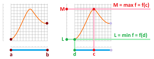
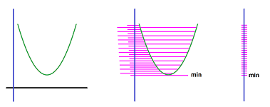
Definition. Given a function $y=f(x)$. Then $x=d$ is called a global maximum point of $f$ on interval $[a,b]$ if $$f(d)\ge f(x) \text{ for all } a\le x \le b;$$ and $x=c$ is called a global minimum point of $f$ on interval $[a,b]$ if $$f(c)\le f(x) \text{ for all } a\le x \le b.$$ (They are also called absolute maximum and minimum points.) Collectively they are all called global extreme points.

Warning: every point of a constant function is both a maximum and a minimum point.

Exercise. Identify extreme points of the functions discussed in this section.

Functions with symmetries

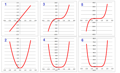
The graphs of some of the functions that we have seen have discernible features. For example, these power functions have symmetries and which ones depend on the degree:

The pieces of paper with the graphs in the second row (even powers) can be folded along the $y$-axis and the left and the right branches will merge. This won't happen with the graphs in the first row (odd powers) even though the two branches seem identical... You'd need to rotate them.

A set has a symmetry if we can transform it into itself via some transformation. More specifically, a subset of the real line or the $xy$-plane has a symmetry if we can transform it into itself via some transformation of the line or the plane, respectively.

Now we are to find the transformations behind the symmetries of these sets on the plane. But, just as in Chapter 3, we start with a line. Remember, all functions are transformations of the line, but we will take only the three simplest:

• shift (translation), $F(x)=x+b$;
• stretch/shrink, $F(x)=kx$; and
• flip (reflection), $F(x)=-x$.

Example. We known that if $n$ and $m$ are integers then so is $n+m$. Therefore, the set of integers ${\bf Z}$ is symmetric with respect to an integer shift. Furthermore, the set of all integer multiples of a fixed real number, say $a$, $$X=\{ka:\ k= … -2,-1,0,1,2,3, ... \},$$ translates into itself when shifted by a multiple of $a$.

$\square$

Example. Because of the same reason -- if $n$ and $m$ are integers then so is $n+m$ -- the set of all integer powers, of a real number, say $a$, $$Y=\{a^k:\ k= … -2,-1,0,1,2,3, ... \},$$ translates into itself when the line is stretched by a power of $a$.

The set $X$ above does not have this symmetry. $\square$

Example. Symmetries relative to the flip are more numerous, in addition to $X$ above:

• $\{0\}$;
• $\{-r,r\}$;
• $(-r,r$;
• $[-r,r]$.

The set $Y$ above does not have this symmetry. $\square$

Now the plane.

Example. These transformations are familiar from using a graphics editor:

$\square$

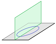
Example. A circle is drawn on a piece of paper and then a piece of glass is put vertically through its center. But, is this a piece of transparent glass or a mirror?

The symmetry is such that we see a circle no matter what. We call it an “axis of symmetry”.

These are a few sets with the axis of symmetry indicated:

As we can see, some sets have more than one axis of symmetry. This is what happens if we put a second mirror (or a transparent glass) on top of a circle drawn on a piece of paper:

$\square$

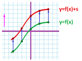
In this section, we will only consider the transformations of the plane that result from transformations of $y$-axis and the $x$-axis, or both, as discussed in Chapter 3. These transformations of the axes produce transformations -- vertical and horizontal respectively. However, our interest here is graphs of functions!

First, a vertical shift. With the exception of $f(x)=0$, the graph of no function will ever be transformed into itself with this shift as it would violate the Vertical Line Test:

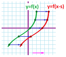
The horizontal shift: $$\newcommand{\ra}[1]{\!\!\!\!\!\xrightarrow{\quad#1\quad}\!\!\!\!\!} \newcommand{\da}[1]{\left\downarrow{\scriptstyle#1}\vphantom{\displaystyle\int_0^1}\right.} \begin{array}{ccc} (x,y)& \ra{ \text{ right } k}& (x+k,y). \end{array}$$

Recall that if the graph of $G$ is the graph of $f$ shifted $k$ units to the right, then $$ G(x) = f(x-k).$$ The new function must be the original one, $f$, for there to be symmetry.

Definition. A function $f$ is called periodic if there is such a $T>0$ that $$f(x+T)=f(x)$$ for all $x$ in the domain of $f$. The smallest such $T$ is called the period of $f$.

Example. In a sense, such a function repeats itself, every $T$. Constant functions are -- trivially -- periodic, for any and every $T$: $$f(x)=c=f(x+T).$$ Examples beyond the trivial are harder to come by, for now. For a function $y=f(x)$ given by a formula, we need to start with $f(x+T)$ and work our way to $f(x)$, identically. For example, no linear polynomial $f(x)=mx+b,\ m\ne 0$, is periodic: $$f(x+T)=m(x+T)+b=mx+mT+b=f(x)+mT\ne f(x),$$ no matter the choice of $T$. We can, however, pick a “sequence”: $$a_n=(-1)^n,$$ defined over all integers.

It is periodic with period $T=1$. Another such function -- with the domain all reals -- is the so-called “fractional part”: $$\{x\}=x-[x].$$

More examples -- trig functions -- will provided in the rest of the chapter. $\square$

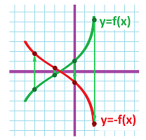
The vertical flip? With the exception of $f(x)=0$, the graph of no function will ever be transformed into itself with this shift as it would violate the Vertical Line Test:

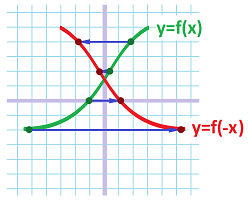
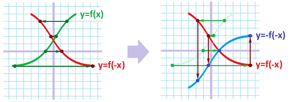
The horizontal flip preserves $x$ and flips the sign of $y$: $$\newcommand{\ra}[1]{\!\!\!\!\!\xrightarrow{\quad#1\quad}\!\!\!\!\!} \newcommand{\da}[1]{\left\downarrow{\scriptstyle#1}\vphantom{\displaystyle\int_0^1}\right.} \begin{array}{ccc} (x,y)& \ra{ \text{ horizontal flip } }& (-x,y). \end{array}$$ So, if the graph of $y = G(x)$ is the graph of $y = f(x)$ flipped horizontally, then $$ G(x) = f(-x). $$

The new function must be the original one, $f$, for there to be symmetry.

Definition. A function is called even if $$ f(-x) = f(x),$$ for all $x$ in its domain.

Example. The graph of $f(x)=x^2$ seems to exhibit this symmetry:

However, we examine the algebra now. For a function $y=f(x)$ given by a formula, we need to start with $f(-x)$ and work our way to $f(x)$, identically. The square power is even: $$f(-x)=(-x)^2=(-x)\cdot (-x)=(-1)x\cdot (-1)x=(-1)(-1)x^2=x^2=f(x).$$ Same for other even powers. The absolute value function is also even: $$|-x|=|x|.$$ The negative part is cancelled, by design. But the cubic power isn't even (a mismatch for every $x\ne 0$): $$f(-x)=(-x)^3=(-x)\cdot (-x)\cdot (-x)=(-1)^3x^3=-x^3\ne x^3=f(x)!$$ $\square$

Exercise. Prove that the circle has this symmetry.

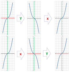
The central symmetry can alternatively be expressed as two consecutive mirror symmetries. Indeed, we just fold the plane in half along the $y$-axis and then along the $x$-axis to make one branch land on top of the other:

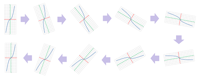
Two of them combined don't give a mirror image anymore; it's understood also as a rotation through $180$ degrees around the origin:

The combination of vertical and horizontal flips flips the signs of both $x$ and $y$: $$\newcommand{\ra}[1]{\!\!\!\!\!\xrightarrow{\quad#1\quad}\!\!\!\!\!} \newcommand{\da}[1]{\left\downarrow{\scriptstyle#1}\vphantom{\displaystyle\int_0^1}\right.} \begin{array}{ccc} (x,y)& \ra{ \text{ horizontal flip } }& (-x,-y). \end{array}$$

So, if the graph of $y = G(x)$ is the graph of $y = f(x)$ flipped horizontally and vertically, then $$ G(x) = -f(-x). $$ The new function must be the original one, $f$, for there to be symmetry.

Definition. A function is called odd if $$ f(-x) = -f(x),$$ for all $x$ in its domain.

Example. The graph of $f(x)=x^3$ seems to exhibit this symmetry:

However, we examine the algebra now. Once again, if we have a formula for a function $y=f(x)$, we need to start with $-f(-x)$ and work our way to $f(x)$, identically. The cubic power is even: $$-f(-x)=-(-x)^3=-(-x)\cdot (-x)\cdot (-x)=-(-1)^3x^3=x^3=f(x).$$ Same for other odd powers. The sign function is also odd: $$-\operatorname{sign}(-x)=\operatorname{sign}(x).$$ The negative part is preserved, by design. But the square power isn't odd (a mismatch for every $x\ne 0$): $$-f(-x)=-(-x)^2=-(-x)\cdot (-x)=-(-1)x\cdot (-1)x=-(-1)(-1)x^2=-x^2\ne x^2=f(x)!$$ $\square$

Exercise. Prove that the circle has this symmetry.

Warning: a random, or a typical, function is neither even nor odd.

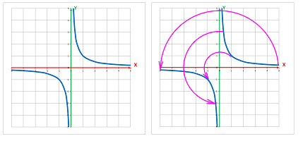
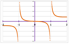
Example. The function $1/x$ seems to have this symmetry:

We can see it in the case of the rest of the reciprocals of the powers, which also confirms the reason for the names:

$\square$

A vertical stretch will not preserve the function except for $f(x)=0$. A horizontal stretch will not preserve the function except for $f$ constant.

Exercise. Is the composition of two functions that are both odd/even odd/even?

Exercise. Half of the graph of an even function is shown below; provide the other half:

Exercise. Half of the graph of an odd function is shown above; provide the other half:

Exercise. Plot the graph of a function that is both odd and even.

Exercise. Is the inverse of an odd/even function odd/even?

Exercise. What is the relation, if any, between these two pairs of properties: (a) even and one-to-one, (b) odd and one-to-one?

Exercise. What transformations of the plane preserve “evenness” and “oddness” of functions?

Quadratic polynomials

In Chapter 2, we thoroughly studied the “square function” $f(x)=x^2$. We now take the idea of squaring the input to the next level and combine it with other algebraic operations. A quadratic polynomial is a function: $$ f(x) = ax^{2} + bx + c, \ a\ne 0. $$ We say that it is presented in the standard form. The numbers $a,b,c$ are the parameters that determine a lot about how the function behaves. We require the first coefficient $a$ to be non-zero to separate the quadratic polynomials from the linear polynomials.

As we saw in Chapter 3, the graph of every quadratic polynomial is made from the “original parabola” of $y=x^2$ via shifting, flipping, and stretching. Some things about this polynomial will be easily deduced from those about the original that we learned in Chapter 2 but others will require some work.

The domain remains the same, all reals, $(-\infty ,+\infty )$. But the values can now be both positive and negative.

The graph shows that it lacks some of the undesirable features: gaps and breaks, corners and cusps.

Different inputs can produce, again, same outputs; quadratic polynomials aren't one-to-one! In fact, a pattern starts to emerge: $$\text{different inputs }\left\{\begin{array}{c} -2\ 10\\ \left\{\begin{array}{c} -1\ 5\\ \left\{\begin{array}{c} \ \ 0\ 2\\ \ \ 1\ 1\\ \ \ 2\ 2\\ \end{array}\right\}\\ \ \ 3\ 5\\ \end{array}\right\}\\ \ \ 4\ 10\\ \end{array}\right\}\text{ same outputs }$$ The inputs/outputs are paired up as the latter start to repeat themselves -- in reverse order -- after we pass $x=1$.

The slopes are still different at different locations.

Furthermore, we know that

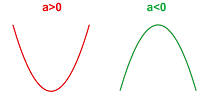
• if $a > 0$, parabola opens up and there is a minimum;
• if $a < 0$, parabola opens down and there is a maximum.

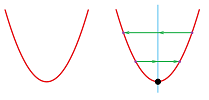
The graph has an axis of symmetry, so that the left branch is a mirror image of the right, but it's not the $y$-axis anymore. To find it we look at other facts first.

Recall that the $x$-intercepts of a function $y=f(x)$ are the real solutions of the equation $f(x)=0$. The following theorem provides the $x$-intercepts of a quadratic polynomial.

THEOREM (Quadratic Formula.) The roots of a quadratic polynomial: $$ f(x) = ax^{2} + bx + c, \ a\ne 0, $$ are given by \begin{array}{|c|}\hline\quad x=\frac{-b\pm\sqrt{b^2-4ac}}{2a}. \quad \\ \hline\end{array}

Exercise. Prove the theorem.

Exercise. Derive Vieta's formulas for the roots $x_1, x_2$ of the quadratic polynomial $ax^2 + bx + c$: $$x_1 + x_2 = -\frac{b}{a}, \quad x_1 x_2 = \frac{c}{a}.$$

In other words, these numbers satisfy the equation: $$ax^{2} + bx + c=0.$$

The formula is frequently written as: $$x_{1,2}=\frac{-b\pm\sqrt{b^2-4ac}}{2a},$$ which means that there are (up to) two solutions: $$x_1=\frac{-b-\sqrt{b^2-4ac}}{2a} \text{ and } x_2=\frac{-b+\sqrt{b^2-4ac}}{2a}.$$ As the solutions to the equation $$f(x) = ax^2 + bx + c=0,$$ these numbers may or may not exist or they might coincide. The formula only produces $x$-intercepts when what's inside the root is non-negative.

Definition. The discriminant of a quadratic polynomial: $$ f(x) = ax^{2} + bx + c, \ a\ne 0,$$ is given by $$D=b^2-4ac.$$

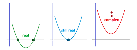
Now, decreasing the value of the discriminant $D>0$ makes the graph of $y=f(x)$ shift upward while the graph has two $x$-intercepts. When $D$ reaches $0$, the graph touches the $x$-axis. Eventually, $D$ becomes negative, the pass the $x$-axis entirely so that the $x$-intercepts disappear:

So, the two $x$-intercepts start to get closer to each other, then merge, and finally disappear. These $x$-intercepts are, respectively: $$\begin{array}{l|lcl} \text{discriminant }&x_1& \quad&x_2\\ \hline D>0&-\frac{b}{2a}-\frac{\sqrt{D}}{2a} &\ne & -\frac{b}{2a}+\frac{\sqrt{D}}{2a}\\ D=0&-\frac{b}{2a} &=& -\frac{b}{2a}\\ D<0& &NONE& \end{array}$$

As a summary, we have the following classification of the roots of quadratic polynomials in terms of the sign of the discriminant.

THEOREM ($x$-intercepts). The two $x$-intercepts of a quadratic polynomial are:

• distinct when its discriminant $D$ is positive;
• equal when its discriminant $D$ is zero;
• absent when its discriminant $D$ is negative.

We will see in Chapter 23 that the last case produces two complex roots.

When the discriminant is zero, we say that the quadratic polynomial is a complete square: $$f(x)=a(x-x_1)^2.$$ It factors in this special way.

Definition. When a quadratic polynomial cannot be factored into linear factors, it is called irreducible.

So, when the discriminant is negative, the polynomial is irreducible.

Now, we know that the axis of a parabola lies half-way between the two $x$-intercepts. Therefore, it is: $$ v =\frac{x_1+x_2}{2}=\frac{1}{2}\left(\frac{-b-\sqrt{b^2-4ac}}{2a} + \frac{-b+\sqrt{b^2-4ac}}{2a}\right)= - \frac{b}{2 a }. $$

The equation $$ y = - \frac{b}{2 a } $$ is the equation of the axis of the parabola.

The formula works even when $D<0$ and there are no $x$-intercepts!

THEOREM (Extrema). Suppose $f(x) = ax^{2} + bx + c,\ a\ne 0,$ is a quadratic polynomial. Then $$v = - \frac{b}{2a}$$ is its extreme point. Moreover,

• $v$ is the global minimum point of $f$ when $a>0$, and
• $v$ is the global maximum point of $f$ when $a<0$.

Definition. The vertex of a parabola is the point on the graph which corresponds to the maximum or the minimum of the function.

THEOREM (Vertex). The $x$-coordinate of the vertex of parabola is $$ v = - \frac{b}{2a}. $$

THEOREM (Range). The range of a quadratic polynomial $y=ax^2+bx+c$ is a closed ray:

• $V=[m,+\infty)$ when $a>0$, and
• $V=(-\infty,M]$ when $a<0$,

where $m$ and $M$ are the minimum and the maximum values of the function respectively.

Exercise. What happens to the graph as we increase $c$? What if we increase $b$? What about $a$?

Polynomial functions

What do linear polynomials $f(x)=mx+b$ and quadratic polynomials $g(x)=ax^2+bx +c$ have in common? There is no division!

Definition. A polynomial is a (numerical) function computed via addition, subtraction, and multiplication only.

No division -- no chance of dividing by zero! We conclude the following.

THEOREM. The domain of a polynomial is the set of all real numbers, ${\bf R}=(-\infty,+\infty)$.

Multiplication include multiplication by constant real numbers as well as by the input, $x$, itself. For example, we might have: $$\begin{array}{lllll} x&\mapsto &\begin{array}{|c|}\hline\quad \text{ add }2 \quad \\ \hline\end{array} & \mapsto & \begin{array}{|c|}\hline\quad \text{ multiply by }2 \quad \\ \hline\end{array} & \mapsto&\begin{array}{|c|}\hline\quad \text{ add } 3\quad \\ \hline\end{array}& \mapsto&\begin{array}{|c|}\hline\quad \text{ multiply by }x \quad \\ \hline\end{array}& \mapsto &...\\ \end{array}$$ This is the formula of this function: $$f(x)=\bigg[\big((x+2)\cdot 2\big)+3\bigg]\cdot x\ ...$$

As an extreme case, it is possible that $x$ might not even appear! Then, in addition to linear and quadratic polynomials, we discover a new class: constant polynomials. Polynomials also include all power functions (if we just keep multiplying by $x$).

The way we learned to understand the linear, $f(x)=mx+b$, and the quadratic polynomials $g(x)=ax^2+bx +c$, was to derive many of their properties from the values of their parameters, or coefficients: $m,b$ and $a,b,c$. There is a standard way to represent a polynomial. For a linear polynomial, it is its “slope-intercept form”. For a quadratic polynomial, the formula $g(x)=ax^2+bx +c$ is the standard form, as opposed to, say, a factored form: $g(x)=a(x-x_1)(x-x_2)$. In order to attack all polynomials this way, we need to put them in a manageable form too. For example, this is how we simplify our formula above: $$f(x)=\bigg[\big((x+2)\cdot 2\big)+3\bigg]\cdot x=\big[(2x+4)+3\big]\cdot x=\big[2x+7\big]\cdot x=2x^2+7x.$$ We can do the same with any polynomial, no matter how many steps are involved.

What is the standard way to represent a polynomial? Let's follow the treatment of the linear and quadratic polynomials and ask: what do they have in common? To make the pattern clear, let's add a constant to the list: $$\begin{array}{ll} \text{constant:}&&&&&5\\ \text{linear:}&&&2x&+&5\\ \text{quadratic:}&3x^2&+&2x& +&5 \end{array}$$ Similar terms are aligned vertically! Accordingly, they have these special names, no matter in what polynomials they appear: $$\begin{array}{ccc} \text{terms:}&\text{quadratic}&&\text{linear}&&\text{constant}\\ &3x^2&+&2x& +&5 \end{array}$$

We add the cubic to the list. We can see the pattern even clearer if we identify the powers of $x$: $$\begin{array}{ll} \text{constant:}&&&&&&&5x^0\\ \text{linear:}&&&&&2x^1&+&5x^0\\ \text{quadratic:}&&&3x^2&+&2x^1& +&5x^0\\ \text{cubic:}&-2x^3&+&3x^2&+&2x^1& +&5x^0\\ \end{array}$$ The powers of $x$ go down all the way to $0$. Furthermore, we progress to the next line by just adding an extra term -- a term of higher power!

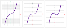
What does it do to the function? Just take a look at the graphs. All linear polynomials a lines and all quadratic polynomials are parabolas. Consider the extra degree of complexity -- three possible shapes of the graph -- that cubic polynomials have:

Definition. The degree of a polynomial is the number $n$ that is the highest power of $x$ present in the formula.

We then start to identify polynomials according their degrees instead of those names: $$\begin{array}{r|cccccccc|lll} \text{degrees}&\quad&3&&2&&1&&0&\\ \hline 0&&&&&&&&5x^0&1\text{ term}\\ 1&&&&&&2x^1&+&5x^0&2\text{ terms}\\ 2&&&&3x^2&+&2x^1& +&5x^0&3\text{ terms}\\ 3&&-2x^3&+&3x^2&+&2x^1& +&5x^0&4\text{ terms}\\ \vdots&&\vdots&&\vdots&&\vdots&&\vdots&\vdots \end{array}$$ As you can see, the terms are also assigned degrees, instead of names.

So, the $n$th degree polynomial will be located in the $(n+1)$st row of the table. It will have $n+1$ terms: $$f(x)=2x^n-11x^{n-1}+...-2x^3+3x^2+2x^1 +5x^0.$$ Here “...” indicates the continuation of the pattern: declining, by $1$, degrees of $x$.

For a general formula, we choose letters to represent the coefficients of the powers of $x$ with the subscripts indicating the power of the corresponding term. It's a finite sequence (familiar from Chapter 1): $$\begin{array}{ll} a_k:\ k=&0&1&2& ... &n-1&n\\ &a_0&a_1&a_2&...&a_{n-1}&a_n \end{array}$$ For the above polynomial, we have: $$\begin{array}{rrr} \text{degrees:}&n&n-1&...&3&2&1&0\\ \text{formula:}&2x^n&-11x^{n-1}&...&-2x^3&+3x^2&+2x^1&+5x^0\\ \text{terms:}&2x^n,&-11x^{n-1},&...&-2x^3,&3x^2,&2x^1,&5x^0\\ \text{coefficients:}&a_n=2,& a_{n-1}=-11,&...&a_3=-2,&a_2=3,&a_1=2,&a_0=5. \end{array}$$

Definition. A polynomial in a standard form is given by a formula: $$ f(x) = a_nx^n+a_{n-1}x^{n-1}+...+a_2x^2+a_1x+a_0, $$ where $a_n,\ a_{n-1},\ ...,\ a_2,\ a_1,\ a_0$ are real numbers called the coefficients of the polynomial. The $n$th term, $a_nx^n$ is called the leading term with the leading coefficient $a_n$. The $0$th term, $a_0$ is called the constant term (or a free term).

Of course, some of these coefficients can be zero but not the leading one, $a_n$; indeed, the degree of a polynomial is the number $n$ that is the highest power of $x$ present in the formula, i.e., $a_n\ne 0$.

What is the meaning of the constant term $a_0$? It's the $y$-intercept: $$\begin{array}{ll} f(0)&=a_nx^n+a_{n-1}x^{n-1}+...+a_2x^2+a_1x+a_0\bigg|_{x=0}\\ &=a_n 0^n+a_{n-1}0^{n-1}+...+a_2 0^2+a_10+a_0\\ &=a_0. \end{array}$$

So, in addition to the definition of polynomials in the beginning of this section, we can say that polynomials are “made” of powers of $x$ (presented Chapter 2) via multiplication by constant coefficients followed by addition: $$f(x)=2x^{3}+4x^{2} -x^2+ 10. $$ $$\begin{array}{ccc} f:& x & \mapsto & \begin{array}{|c|}\hline &\begin{array}{lllll} x&\mapsto &\begin{array}{|c|}\hline\quad \text{ cube it } \quad \\ \hline\end{array} & \mapsto & \begin{array}{|c|}\hline\quad \text{ multiply by }2 \quad \\ \hline\end{array} & \mapsto\\ x&\mapsto &\begin{array}{|c|}\hline\quad \text{ square it } \quad \\ \hline\end{array} & \mapsto & \begin{array}{|c|}\hline\quad \text{ multiply by }3 \quad \\ \hline\end{array} & \mapsto\\ x&\mapsto &\begin{array}{|c|}\hline\quad \text{ pass it } \quad \\ \hline\end{array} & \mapsto & \begin{array}{|c|}\hline\quad \text{ multiply by }-1 \quad \\ \hline\end{array} & \mapsto\\ x&\mapsto &\begin{array}{|c|}\hline\quad \text{ choose }10 \quad \\ \hline\end{array} & \mapsto & \begin{array}{|c|}\hline\quad \text{ pass it } \quad \\ \hline\end{array} & \mapsto\\ \end{array}& \begin{array}{|c|}\hline\quad \text{ add } \quad \\ \quad \text{ them } \quad \\\hline\end{array}& \mapsto & y\\ \hline \end{array} & \mapsto & y \end{array}.$$

We will see that, when zoom out from, the graphs of polynomials resemble those of the power functions but, when zoomed in, there may be many $x$-intercepts:

We have learned from our experience with linear and, especially, quadratic polynomials that there is another, just as important form for a polynomial: the factored form. For example, a linear polynomial is factored: $$f(x)=mx+b=m\left( x+\frac{b}{m}\right),\ m\ne 0.$$ The factor in parentheses is a generic linear factor. Why not the original, also linear, polynomial as a factor? The new factor has a special importance because we can read something important directly from it:

• $x=-\frac{b}{m}$ is the $x$-intercept of $f$.

Next, suppose a quadratic polynomial happens to have two real roots $x_1$ and $x_2$. They come from the Quadratic Formula. They give us two (or one if equal) $x$-intercepts and two (possibly equal) factors: $$f(x)=ax^2+bx+c=a(x-x_1)(x-x_2).$$ We see how the standard form is converted to the factored form with two linear terms. When the two roots are equal, $x_1=x_2$, we have a complete square: $$f(x)=a(x-x_1)(x-x_1)=a(x-x_1)^2.$$ The $x$-intercepts coincide and so do the two factors. Furthermore, an irreducible quadratic polynomial, such as $x^2+1$, has no $x$-intercepts nor linear factors! We say that there is one -- irreducible quadratic -- factor.

Treating as polynomials,

• the linear factors have degree $1$, while
• the quadratic factors have degree $2$.

It is important to note that the sum of the degrees of the factors of a quadratic polynomial remains $2$.

We will use the following analogy to better understand factoring polynomials. $$\begin{array}{r|l} \text{Integers}&\text{Polynomials}\\ \hline \text{The sum and the product of two integers }&\text{The sum and the product of two polynomials }\\ \text{is an integer.}&\text{is a polynomial.}\\ \hline \text{A prime number cannot be further }&\text{An irreducible polynomial cannot be further }\\ \text{factored into smaller integers }> 1. & \text{factored into lower degree polynomials.} \\ 2,3,5,7,11,13, ... & x-1,x+2,x^2+1, ...\\ \hline \text{Fundamental Theorem of Arithmetic:}&\text{Fundamental Theorem of Algebra:}\\ \text{Every integer can be represented as}&\text{Every polynomial can be represented as}\\ \text{the product of primes.}&\text{the product of irreducible factors.}\\ \hline \text{This representation is unique,}&\text{This representation is unique,}\\ \text{up to the order of the factors.}&\text{up to the order of the factors.}\\ q=2^5\cdot 3^2\cdot 5^1\cdot...&Q=(x-1)^5\cdot (x+2)^2\cdot (x^2+1)\cdot...\\ \text{Its multiplicity is how many times it appears.}&\text{Its multiplicity is how many times it appears.}\\ \hline &\text{Irreducible polynomials have degrees }1 \text{ and } 2.\\ &\text{The sums of the degrees of the factors of }\\ &\text{a polynomial of degree }n\text{ is }n. \end{array}$$

It is the purpose of the factored form to display the $x$-intercepts. The fact that we can see them follows from this fundamental result about numbers.

THEOREM (Zero Factor Property). If the product of two numbers is zero then either one of them or both is zero too. Conversely, if either one of the two numbers is zero, then so is their product.

In other words, we have: $$a=0\ \texttt{ OR }\ b=0\ \Longleftrightarrow\ ab=0.$$ Then substituting $x=x_1$ into the linear polynomial $x-x_1$ makes it equal to zero -- as well as any polynomial that has it as a factor!

THEOREM (Linear Factor Theorem). A linear factor $(x-x_1)$ is present in the factorization of a polynomial $P$ if and only if $x=x_1$ is an $x$-intercept of $P$.

Warning: the problem of how to factor a higher degree polynomial has no complete solution.

We have a correspondence: $$\begin{array}{|c|}\hline \quad \text{factor }(x-x_1)\ \longleftrightarrow\ x\text{-intercept } x=x_1. \quad \\ \hline\end{array}$$

Example. Consider the polynomial: $$Q(x)=x(x-1)^5\cdot (x+2)^2\cdot (x-.5)\cdot(x^2+1)\cdot...$$ It has $x$-intercepts corresponding to each of its linear factors, as follows: $$\begin{array}{rcccc} x\text{-intercepts:}&0&1& -2&.5&...\\ \text{points on the graph:}&(0,0)&(1,0)&(-2,0)&(.5,0)&...\\ \end{array}$$ The quadratic factor doesn't contribute anything because it remains positive for all $x$. If we arrange the values of $x$, we can see what the $x$-axis looks like with the four points of the graph shown: $$\begin{array}{rcccc} x\text{-axis:}&-&\bullet&\bullet& \bullet&\bullet&...&\to\ x\\ &&-2&0&.5&1&...\\ \end{array}$$ $\square$

In other words, solving a polynomial equation $P(x)=0$ and factoring the polynomial $P$ is the same thing... except the former doesn't care about the multiplicities!

Recall what we know about the power functions, $x,\ x^2, x^3,\ ...$ (Chapter 2):

The graphs reveal that the nature of an $x$-intercept depends on its multiplicity:

• if the multiplicity of a linear factor is odd, the graph crosses the $x$-axis (upward or downward);
• if the multiplicity of a linear factor is even, the graph touches the $x$-axis (from above or from below).

Example. We continue with the last example. We assume that the rest of the factors of our polynomial are irreducible and positive: $$Q(x)=x(x-1)^5\cdot (x+2)^2\cdot (x-.5)\ \cdot(x^2+1)\cdot...$$ The $x$-intercepts and their multiplicities are listed below and they tell us how the graph interacts with the $x$-axis: $$\begin{array}{rccc} x\text{-intercepts:}&0&1& -2&.5\\ \text{multiplicities:}&1&5& 2&1\\ \text{graph:}&\text{cross}&\text{cross}&\text{touch}&\text{cross}&\\ \text{options:}&\searrow&\searrow&\smile&\searrow\\ \text{options:}&\nearrow&\nearrow&\frown&\nearrow\\ \end{array}$$ There are two options for each $x$-intercept though... To find which one appears, we pick a starting point for the graph! How about $x=-10$? We substitute and discover that $Q(-10)<0$. Therefore, there is a point to the left of the first $x$-intercept, $x=-2$, that lies below the $x$-axis. It follows that we must cross the axis upward at $x=-2$! Now we are above the $x$-axis. Therefore, we must cross the axis downward at $x=0$! And so on. We order the $x$-intercepts and go from left to right discovering which way we cross the axis at each $x$-intercept as soon as we reach it: $$\begin{array}{rccc} x\text{-values:}&-10&-2&0&.5&1& \\ y\text{-values:}&-&0&0& 0&0&\\ \text{graph:}&&\text{cross}&\text{cross}&\text{touch}&\text{cross}&...\\ &&\nearrow&\searrow&\frown&\nearrow\\ \end{array}$$ We have a rough sketch of the graph:

$\square$

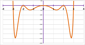
Example (plotting). We can avoid using the multiplicities... Let's analyze this polynomial: $$\begin{array}{lll} f(x)&=(x^4-9x^2)(x^2-4)^2(3x^2+2)&\text{ ...we need to further factor it! }\\ &=x^2(x-3)(x+3)(x-2)^2(x+2)^2\ \cdot(3x^2+2). \end{array}$$ With only linear factors listed, we can see the $x$-intercepts. They are simply read off the list of linear factors: $$x=0,\ 3,\ -3,\ -2,\ 2.$$ At these points and at these points only the function may change its sign. We now list all the factors. They are simple enough for us to determine where and whether they change their signs: $$\begin{array}{r|ccc} \text{factors }& \text{ signs }\\ \hline x^2&+&+&+&+&+&0&+&+&+&+&+\\ x-3&-&-&-&-&-&-&-&-&-&0&+\\ x+3&-&0&+&+&+&+&+&+&+&+&+\\ (x-2)^2&+&+&+&+&+&+&+&+&+&+&+\\ (x+2)^2&+&+&+&+&+&+&+&+&+&+&+\\ \hline \text{domain }&\cdots&\bullet&\cdots&\bullet&\cdots&\bullet&\cdots&\bullet&\cdots&\bullet&\cdots&\to x\\ x=&&-3&&-2&&0&&2&&3\\ \hline f(x)=&+&0&-&0&-&0&-&0&-&0&+\\ &\searrow&0&\smile&0&\smile&0&\smile&0&\smile&0&\nearrow \end{array}$$ Here we went vertically in each column and determined the sign of the function using: $+\cdot-=-$, etc. An idea of what the graph of $f$ looks like is seen in the last row: it crosses the $x$-axis downward, then touches it three times from below, and then crosses it upward. We can sketch the graph based on the last row only:

The table solves for us this equation and these inequalities: $$f(x)=0,\ f(x)>0,\ f(x)\ge 0,\ f(x)<0,\ f(x)\le 0.$$ We confirm our analysis with a graphic utility:

$\square$

Example. This is what happens when one solves a polynomial inequality when the polynomial is already factored:

$\square$

Rational functions

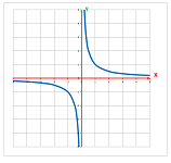
We are already familiar with such an important function as the reciprocal, $$y=\frac{1}{x}.$$

Even with such a simple formula, once division is introduced, the complexity of a function increases dramatically. We can see some new --in comparison to the polynomials -- features in the graph.

First, holes in the domain appear. As we see above, the hole in the domain corresponds to a vertical line on the $xy$-plane that the graph can't intersect! As the curve approaches this line, it has to start to climb, faster and faster, up or down. The result is a graph with a virtually vertical part close to this line. These lines are called vertical asymptotes.

An opposite -- but also very similar -- behavior is seen along a certain horizontal line. If the graph can't cross it, it has to start to crawl, with virtually no up or down progress. Such a line is called a horizontal asymptote.

If we zoom out, the ends of the graph merge with the asymptotes. The topic of asymptotes is fully developed in in Chapter 6.

Warning: a rational function doesn't have to have asymptotes.

Example. What is the domain of $$f(x)=\dfrac{x - 1}{x + 1}?$$ We look at the denominator, set it equal to zero, $x + 1 = 0$, and solve for $x$. Then, $x = -1$ is not in the domain and the rest of the real numbers are.

$\square$

As we discovered in the last section, the algebra of polynomials mimics the algebra of integers. We take this idea to the next level and observe that the rational functions appear from polynomials -- just like the rational numbers from integers -- via division! We continue with our analogy from the last section. $$\begin{array}{r|l} \text{Integers}&\text{Polynomials}\\ \hline \text{The sum and the product of two integers }&\text{The sum and the product of two polynomials }\\ \text{is an integer.}&\text{is a polynomial.}\\ \hline \text{The ratio of two integers} &\text{The ratio of two polynomials}\\ \text{is called a rational number.} & \text{is called a rational function.} \\ \hline \text{The sum, the product, and the ratio}&\text{The sum, the product, and the ratio }\\ \text{ of two rational numbers is a rational number.}&\text{of two rational functions is a rational function.}\\ \frac{2}{3}+\frac{1}{2}=\frac{7}{3\cdot 2}&\frac{x}{x-1}+\frac{1}{x+1}=\frac{x^2+2x-1}{(x-1)(x+1)}\\ \hline \text{The numerator and the denominator of every}&\text{The numerator and the denominator of every}\\ \text{rational number can be represented as}&\text{rational function can be represented as}\\ \text{the products of different primes.}&\text{the products of different irreducible factors.}\\ \frac{p}{q}=\frac{2^5\cdot 5^2\cdot 7^1\cdot...}{3^2\cdot 11^2\cdot ...}&\frac{P}{Q}=\frac{(x-1)^5\cdot (x+2)^2\cdot (x^2+1)\cdot...}{(x+1)^2\cdot (x-3)^1\cdot (2x^2+1)\cdot...}\\ \end{array}$$

Warning: cancelling factors will simplify the rational function, but it won't (and must not) change its domain.

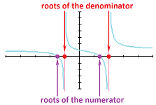
How do we find the $x$-intercepts of a rational function? We know all we need to know. Just as in the last section, we use the fact, called the Linear Factor Theorem, that substituting $x=x_1$ into the linear polynomial $x-x_1$ makes it equal to zero -- as well as any polynomial that has it as a factor. We conclude the following.

THEOREM. A rational function's $x$-intercepts

• are the roots of its numerator, provided they
• aren't also among the roots of the denominator.

Warning: All polynomials are rational functions too.

How do we find the implied domain of a rational function? We use the Linear Factor Theorem again.

Example. What is the domain of $$ f(x) = \frac{x - 1}{x^{2} - 4}? $$ Set the denominator to $0$ and solve: $$\begin{array}{rl} x^{2} - 4 & = 0, \\ x^{2} & = 4, \\ x & = \pm 2. \end{array}$$ So, the domain consists of all real numbers except $\pm 2$: $$\text{domain }=\{x:\ x\ne \pm 2\}=(-\infty,-2)\cup (-2,2)\cup (2,+\infty).$$ $\square$

The challenge of plotting rational functions is that the holes in the domain break the graph into separate branches.

Example. Consider the rational function: $$f(x)=\frac{x^2\cdot (x+2)\cdot (x-1)\cdot(x^2+1)}{(x+1)\cdot(x-3)^2 \cdot(x^2+2)}.$$ We analyze these two polynomials separately and derive two separate sets of information about the function: $$\begin{array}{r|rccc} \text{from the numerator...}&x\text{-intercepts:}&-2&&0&1&\\ \hline \text{from the denominator...}&\text{asymptotes:}&&-1&&&3&\\ \end{array}$$ The quadratic (irreducible) factors don't contribute anything. This is what the $x$-axis looks like with the three points of the graph and two holes in the domain shown: $$\begin{array}{rccc} x\text{-axis:}&-&\bullet&\circ& \bullet&\bullet&\circ&...&\to\ x\\ &&-2&-1&0&1&3&\\ \end{array}$$ The numerator's roots and their multiplicities tell us whether the graph passes across the $x$-axis or stays on the same side: $$\begin{array}{rccc} x\text{-intercepts:}&-2&0&1\\ \text{multiplicities:}&1&2& 1\\ \text{graph:}&\text{cross}&\text{touch}&\text{cross}&\\ \end{array}$$ The denominator's roots and their multiplicities tell us whether the graph jumps over the $x$-axis or stays on the same side: $$\begin{array}{rccc} \text{asymptotes:}&-1&3\\ \text{multiplicities:}&1&2\\ \text{graph:}&\text{jump}&\text{stay}&\\ \end{array}$$ There are still two options for each of these points. Just as in the last section, we need a starting point and choose $x=-10$. Since $f(-10)<0$, we have a point to the left of the left-most $x$-intercept, $x=-2$, that lies below the $x$-axis. It follows that we must cross the $x$-axis upward at $x=-2$. After that we are above the $x$-axis and the process continues: $$\begin{array}{rccc} x\text{-values:}&-10&-2&-1&0&1&3& \\ \text{graph:}&-&\bullet&\circ&\bullet&\bullet&\circ&\\ \text{graph:}&&\text{cross}&\text{jump}&\text{touch}&\text{cross}&\text{stay}\\ &&&\nearrow\quad&&&\nearrow\nwarrow\\ x-\text{axis:}&&\nearrow&\vdots&\frown&\nearrow&\vdots&\\ &&&\quad\swarrow&&&\\ \end{array}$$ The bottom of the table is meant to visualize the date that we have collected. Furthermore, here is a rough sketch of the graph based on this data:

We can also derive solutions of the inequalities for the function from this sketch. For example, for the inequality $$f(x)>0,$$ the solution set is $$(-2,-1)\cup (1,3)\cup (3,+\infty).$$ And so on. $\square$

Exercise. Write the solution sets for the inequalities: $$f(x)\ge 0,\ f(x)<0,\ f(x)\ge 0.$$

Example. We can avoid using multiplicities in this way. Let's analyze this rational function: $$f(x) = \frac{x(3x^{2} + 1)}{(x-1)(x+1)}.$$ First, the domain is all reals except $x=\pm 1$. We now need find the signs of the factors and then the signs of the function. We take note of the domain and list all the factors present. We then determine where each of them is equal to zero and how its signs changes with $x$ as it passes this location. Finally, we find the sign of $f(x)$ as it varies with $x$, one interval at a time. It is done in the same manner as for polynomials because the weather we multiply or divide, the sign of the term affects the result the same: $$(+)\cdot(+)=(+) \ \text{ or }\ (+)/(+)=(+),\quad (+)\cdot(-)=(-) \ \text{ or }\ (+)/(-)=(-),$$ and so on. These are the results: $$\begin{array}{r|ccc} \text{factors }& \text{ signs }\\ \hline x&-&-&-&0&+&+&+\\ 3x^{2} + 1 &+&+&+&+&+&+&+\\ x-1 &-&-&-&-&-&0&+\\ x+1 &-&0&+&+&+&+&+\\ \hline x\text{-axis}&&\circ&&\bullet&&\circ&& \longrightarrow x\\ x=&&-1&&0&&1&&\\ \hline f(x)&-&\vdots&+&0&-&\vdots&+\\ \end{array}$$ We confirm the result by plotting:

We can also derive solutions of the inequalities from the table. For example, for the inequality $$f(x)\le 0,$$ the solution set is $$(-\infty,-1)\cup [0,1).$$ And so on. $\square$

This is the summary of where the information about the graph of a rational function comes from:

Furthermore, this is the summary of what happens when we solve a rational inequality (and the equation), when the function comes already factored:

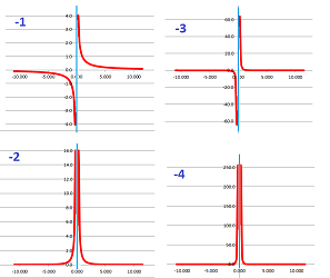
Example. So, the domain is entirely determined by the roots of the denominator of the rational function, $f(x)=P(x)/Q(x)$. What about the range? The example of the negative powers -- $P(x)=1,\ Q(x)=x^n$ -- shows the scope of possibilities:

So,

• if $n$ is odd, the range of $\frac{1}{x^n}$ is $(-\infty,0)\cup (0,+\infty)$;
• if $n$ is even, the range of $\frac{1}{x^n}$ is $(0,+\infty)$.

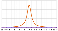
The example of $f(x)=\frac{1}{x^2+1}$ shows that the range doesn't have to be infinite:

$\square$

The root functions

We have applied the following operations to the power functions, $x,\ x^2,\ x^3,\ …$:

• addition and subtraction, producing polynomials;
• multiplication, producing more power functions and more polynomials;
• division, producing the reciprocals of powers and the rational functions;
• composition, producing more power functions.

What if -- in addition to these operations -- we also consider the inverses of the power functions?

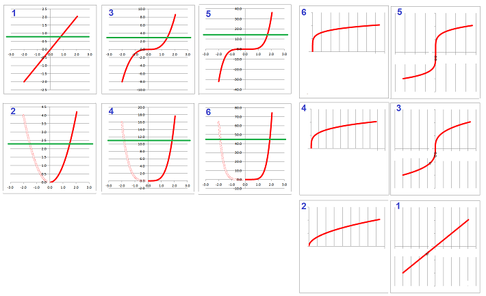
Following our experience with $y=x^2$, we do this all at once. It is a flip of the graphs about the line $y=x$:

The even degree powers aren't one-to-one! To make them invertible, we cut their domains, and codomains, to $[0,+\infty)$:

• the square root, $y=\sqrt{x}$, is the inverse of $x=y^2,\ x,y\ge 0$;
• the cubic root, $y=\sqrt[3]{x}$, is the inverse of $x=y^3$;
• the fourth degree root, $y=\sqrt[4]{x}$, is the inverse of $x=y^4,\ x,y\ge 0$;
• ...
• the $n$th degree root, $y=\sqrt[n]{x}$, is the inverse of $x=y^n$ with domain $x,y\ge 0$ when $n>1$ is even;
• ...

The definition below is just another way to say the same.

Definition. For a real number $x$, the $n$th root of $x$ is such a number $y$ that $y^n=x$, denoted by: $$y=\sqrt[n]{x}.$$

In other words, $y$ is a solution of the equation $y^n=x$. We imagine that we have solved all of these equations, for all values of $y$...

The symbol $\sqrt{\quad}$ is also known as the radical.

Example. Consider the function $$ \sqrt{ x - \sqrt{x}}. $$ This is its diagram: $$\begin{array}{ccc} f:& x & \mapsto & \begin{array}{|c|}\hline &x& \begin{array}{lcccl} \nearrow &x &\mapsto &x & \mapsto & x & \searrow\\ \\ \searrow &x &\mapsto &\begin{array}{|c|}\hline\quad \sqrt{\quad} \quad \\ \hline\end{array} & \mapsto & u & \nearrow\\ \end{array}& \begin{array}{|c|}\hline\quad - \quad \\ \hline\end{array} \mapsto & z \\ \hline \end{array} & \mapsto & z \end{array}$$ Find the domain. Whatever is inside the square root can't be negative. So, we need to find all $x$ for which

• first, $x \geq 0$, i.e., $x$ is positive; and
• second, $x - \sqrt{x} \geq 0$.

Solve it: $$ x \ge \sqrt{x} \ \Longrightarrow\ x^{2} \geq x \ \Longrightarrow\ x \geq 1.$$ The domain is $$D = [1, \infty). $$ $\square$

Exercise. Find the inverse of the function above and its domain.

Example. Given $$ y = \sqrt{u} + \sqrt{4 - u},$$ find the domain, i.e., find all $u$'s for which the formula makes sense. Make sure that $\sqrt{\, ?\,}$ makes sense, i.e., what's inside cannot be negative.

• $\sqrt{u}\ \Longrightarrow\ u \geq 0$;
• $\sqrt{4 - u} \ \Longrightarrow\ 4 - u\ge 0\ \Longrightarrow\ u \leq 4$.

Each $u$ in the domain must satisfy both inequalities, $$u \geq 0\ \texttt{ AND }\ u \leq 4.$$ Hence, the domain is: $$ D = [0,4]. $$ $\square$

Exercise. Find the inverse of the function above and its domain.

The illustration above suggests the following.

THEOREM. The roots of odd degrees have the domain and range equal to $(-\infty,+\infty)$. They are also increasing, one-to-one, and odd.

THEOREM. The roots of even degrees have the domain and range equal to $[0,+\infty)$. They are also increasing, one-to-one, and not even.

Exercise. Prove the theorems.

We turn to algebra...

Because the roots are the inverses of the power functions, their algebraic properties are parallel. For example, we can “distribute” powers (in other words, exponents, as discussed in Chapter 1) over multiplication: $$A^n\cdot B^n=(A\cdot B)^n.$$ As it turns out, we can also “distribute” roots over multiplication, as follows.

THEOREM (Products of Roots). For any integer $n$, we have: $$\sqrt[n]{a\cdot b}=\sqrt[n]{a}\cdot \sqrt[n]{b}$$ provided $a,b\ge 0$ whenever $n$ is even.

Proof. We use the properties of the integer exponents (repeated multiplication) presented in Chapter 1. Suppose $$A=\sqrt[n]{a},\quad B= \sqrt[n]{b}.$$ Then, $$a=A^n,\quad b=B^n.$$ Therefore, $$ab=A^n\cdot B^n=(AB)^n.$$ Hence, $$\sqrt[n]{ab}=AB.$$ $\blacksquare$

Warning: we can't “distribute” roots -- nor powers -- over addition ($\sqrt[n]{a+b}\ne ...$).

Furthermore, we know that the powers (exponents) are multiplied when composed: $$\left( Q^n \right)^m=Q^{n \cdot m}.$$ The same happens with the degrees of roots.

THEOREM (Compositions of Roots). For any integers $n$ and $m$, we have: $$\sqrt[n]{\sqrt[m]{a}}=\sqrt[nm]{a},$$ provided $a\ge 0$ when $n$ or $m$ is even.

Proof. We use the properties of the integer exponents (repeated multiplication) presented in Chapter 1. Suppose $$A=\sqrt[m]{a},\quad Q= \sqrt[n]{A}.$$ Then, $$a=A^m,\quad A=Q^n.$$ Therefore, $$Q^{nm}=\left( Q^n \right)^m=\left( A \right)^m=a.$$ Hence, $$\sqrt[nm]{a}=Q.$$ $\blacksquare$

These theorems will be used later in this chapter to prove that every root can be seen as a (fractional) power, the reciprocal of the power the root came from.

The exponential function

Recall what we learned about the algebra of exponents in Chapter 1. This is the summary of what we know (arbitrary $a,b$): $$\begin{array}{r|rl|rl} \text{}&\text{Multiplication:}&&\text{Exponentiation:}\\ \hline \text{Conventions: }x=1,2, ... &\underbrace{a+a+a+ ... +a}_{x\text{ times}}&=a\cdot x&\underbrace{a\cdot a\cdot a\cdot ... \cdot a}_{x\text{ times}}&=a^x\\ \hline x=0 & a\cdot 0 & =0 & a^0&=1\\ \hline x=-1,-2, ... &ax&= (-a)(-x) & a^x & =\left(\frac{1}{a}\right)^{-x}=\frac{1}{a^{-x}}\\ \hline \text{Rules: }\ 1.&a (x+y)&=a x+a y & a^{x+y}&=a^x a^y\\ \hline 2.&(a+b) x&=a x+b x & (a b)^x & = a^x b^x\\ \hline 3.&a(x y)&=(a x) y & a^{x y}&=(a^x)^y\\ \hline \end{array}$$

This is just a review of how the power -- including the reciprocal powers -- functions operate. However, our current interest is a different kind of function... Recall the notation and the terminology: $$\begin{array}{rl} &\text{exponent}\\ &\downarrow\\ &\small{n}\\ a\\ \uparrow\\ \text{base} \end{array}$$

Definition. The exponential function of base $a$ is defined to be: $$f(x)=a^x,$$ with the domain the set of all integers: $${\bf Z}=\{... ,-3,-2,-1,0,1,2,3, ...\}.$$

Warning: in contrast to the power functions $x^n$ with a variable base, this is a function, $a^x$, with a variable exponent.

Note that our analogy between the arithmetic progression and the geometric progression has become the one between the linear function (left) and the exponential function (right).

The domain misses some of the numbers that interest us!

Example. Suppose bacteria double in number every day starting with $1$. What happens after $10.5$ days? $$x=10.5, \quad 2^{10.5} = ?$$ $\square$

The domain of the exponential function $y=a^x$ with base $a>0$ is all integers. What do we do about these gaps? Can, or should, we fill them, in a meaningful manner?

Example (compounded interest). Consider what happens to a $\$1000$ deposit with $10\%$ annual interest, compounded yearly (Chapter 1): $$ \begin{aligned} \$ 1000, 1000 \cdot 1.10 & = 1000 + 10\% \textrm { of } 1000 \\ \textrm{begin, after 1 year } & = \textrm{ principal } + \textrm{ interest} \\ & = 1000 + 1000 \cdot .10 \\ & = 1000(1 + 0.1 ) \\ & = 1000 \cdot 1.1 . \end{aligned}$$ Therefore, after $x$ years we have: $$f(x)=1000\cdot 1.1^{x}.$$ where $x$ is a positive integer. But how much do I have if the interest is also compounded in the middle of the year? The amount has grown by such a proportion, say $r$, that, if applied again, will give me the same ten percent growth! In other words: $$f(.5)=1000\cdot r \text{ and } r\cdot r=1.1.$$ Therefore, $$r=\sqrt{1.1}.$$ It seems we will have to take roots. $\square$

Exercise. If your bank will pay you $10\%$ for the first year and $5\%$ for the second, what single interest can it offer to pay you as much over the two years? Explain the meaning of the average interest rate.

The analogy with the linear function is as follows.

• Question: how do you add $a$ in two steps? Answer: add $\frac{a}{2}$ twice.
• Question: how do you multiply by $a$ in two steps? Answer: multiply by $\sqrt{a}$ twice.

So, we choose a new convention.

Definition. For any positive integer $n$, we set the reciprocal power to be: $$a^{1/n}=\sqrt[n]{a}. $$

Exercise. Show that Rules 2 and 3 above still hold.

We would like to have the exponential function $y=a^x$ to defined for all $x$, i.e., domain = $(-\infty, \infty)$. So far, $a^{x}$ is defined only if $x$ is an integer (and $a>0$). Can exponents be fractional? We have a new convention.

Definition. If $x=\frac{m}{n}$, where $m,n$ are integers with $n>0$, then the rational power is defined to be: $$\begin{array}{|c|}\hline \quad a^\frac{m}{n}=\sqrt[n]{a^m}. \quad \\ \hline\end{array}$$

Warning: in contrast to geometric progressions, the exponential functions can only have positive base, $a>0$; no $(-1)^{x}$ anymore.

We now need to show that the rules still apply to all rational numbers.

THEOREM (Rules of Exponents). The rules 1-3 below are satisfied for all rational $x$ and $y$: $$\begin{array}{ll} 1.& a^{x+y}&=a^x a^y;\\ 2.& a^x b^x&=(a b)^x;\\ 3.& a^{x y}&=(a^x)^y.\\ \end{array}$$

Proof. Suppose $x=\frac{1}{n}$, where $n$ is a positive integer. Then, $$a^x b^x= a^\frac{1}{n}b^\frac{1}{n}=\sqrt[n]{a}\sqrt[n]{b} =\sqrt[n]{ab}=(ab)^\frac{1}{n} =(ab)^x,$$ according to the Product of Roots theorem in the last section. We have Rule 2 for the reciprocals.

Suppose $x=\frac{1}{n}$ and $y=\frac{1}{m}$, where $n,m$ are positive integers. Then, $$(a^x)^y = \left( a^\frac{1}{n} \right)^\frac{1}{m} =\sqrt[m]{\sqrt[n]{a}}=\sqrt[nm]{a} = a^\frac{1}{nm}= a^{\frac{1}{n}\frac{1}{m}}=a^{xy},$$ according to the Composition of Roots theorem in the last section. We have Rule 3 for the reciprocals.

Suppose $x=\frac{m}{n}$, where $m$ is an integer and $n$ is a positive integer. Then, $$a^x b^x= a^\frac{m}{n}b^\frac{m}{n}=\sqrt[n]{a^m}\sqrt[n]{b^m} =\sqrt[n]{a^mb^m}=\left( (ab)^m\right)^\frac{1}{n} =(ab)^\frac{m}{n} =(ab)^x,$$ according to Rule 2 for the reciprocals. We have Rule 2 . $\blacksquare$

Exercise. Provide the missing parts of the proof.

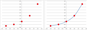
What does the graph of this new function look like? One can imagine that, as these fractions get larger and larger denominators, the domain is becoming denser and denser:

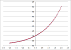
Eventually, these initially loose points seem to form a curve!

After all, the domain contains all rational numbers ${\bf Q}$ and the rational numbers are so dense that any interval, no matter how small, will contain infinitely many of them. Therefore, there are no gaps in the graph! However, its points remain disconnected from each other; a little blow and the curve falls apart:

Indeed, the points on the graph with irrational $x$-coordinates are missing: $$x= \sqrt{2},\ \sqrt{3},\ \pi .$$ And the irrational numbers are so dense that any interval, no matter how small, will contain infinitely many of them. So, even though there are no gaps in the graph, there are invisible “cuts” everywhere! We can define the function for the irrational exponents by “approximating” them with rational numbers, as presented in Chapter 5. For example, the sequence $2^3,\ 2^{3.1},\ 2^{3.14},\ ...$ will approximate $2^\pi$. The three rules are still to be obeyed.

Warning: even though this function has been built from the power functions and the roots, it's very different from them.

This is the summary of our conventions ($a>0$ real, $m,n$ positive integers): $$\begin{array}{c|l|rl|rl} \text{}&&\text{Multiplication:}&&\text{Exponentiation:}\\ \hline 1. &x=1,2, ... &ax&=\underbrace{a+a+a+ ... +a}_{x\text{ times}}&a^x&=\underbrace{a\cdot a\cdot a\cdot ... \cdot a}_{x\text{ times}}\\ \hline 2. &x=0 & a\cdot 0 & =0 & a^0&=1\\ \hline 3. &x=-1,-2, ... &ax&= (-a)(-x)=-a(-x) & a^x & =\left(\frac{1}{a}\right)^{-x}=\frac{1}{a^{-x}}\\ \hline 4. &x=\frac{m}{n}&ax&=\frac{am}{n}=\frac{a}{m}n & a^x & =\sqrt[n]{a^m}=\left(\sqrt[n]{a}\right)^m\\ \hline 5. &x\text{ real}&&&& \text{still to come...} \end{array}$$

Below, we assume that the exponential function is defined for all real numbers!

Let's collect some facts about this function from its graph.

THEOREM. The exponential function $y=a^x$ with base $a>0$ satisfies the following:

• the domain is $(-\infty,+\infty)$;
• the range is $(0, \infty)$;
• the $y$-intercept is $(0, 1)$;
• there are no $x$-intercepts.

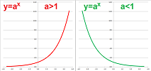
THEOREM (Monotonicity of Exponent). The exponential function with base $a > 0$ satisfies the following: $$ \begin{aligned} y=a^{x} & \textrm{ is increasing if } a > 1, \\ y=a^{x} & \textrm{ is decreasing if } a < 1. \end{aligned} $$

Proof. Suppose $a>1$. The theorem has already been proven for the case of integer $x$. Now, suppose $x$ and $y$ are rational numbers and $x<y$. Suppose

• $x=n/m$ for two integers $m,n$, and
• $y=p/q$ for two integers $p,q$.

Then $n/m<p/q$, or $nq<mp$. Then $a^{nq}<a^{mp}$, because the exponential function is increasing for integer inputs. Therefore, $\sqrt[q]{a^{nq}}<\sqrt[q]{a^{mp}}$, because roots are increasing functions. Then, $a^{n}<a^{mp/q}$. Similarly, $\sqrt[m]{a^{n}}<\sqrt[m]{a^{mp/q}}$, or $a^{n/m}<a^{p/q}$. $\blacksquare$

These two behaviors are called, respectively,

• “exponential growth” (population growth, compounded interest), and
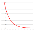
• “exponential decay” (population decline, radioactive decay, warming and cooling).

Corollary. The exponential function is one-to-one and, therefore, invertible.

The inverse is discussed in the next section.

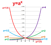
Within the two classes, the exponential functions still vary according to their bases: the larger $a$ is, the faster $a^x$ grows (to be considered in Chapter 7):

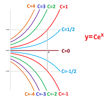
The constant function separates the exponential growth functions from the exponential decay functions.

There are more patterns to discover about these functions.

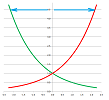
Example. Let's plot $$y=\frac{1}{2^x}.$$ We save time by making an observation: $$\frac{1}{2^x}=2^{-x}.$$ Therefore, the graph of our function (green) is that of $y=2^{x}$ (red) flipped about the $y$-axis:

We can also notice this: $$\frac{1}{2^x}=\left(\frac{1}{2}\right)^{x}.$$ This is also an exponential function! Its base is $1/2$ the reciprocal of that of the original. $\square$

The lesson is that the graph of the exponential function of base $a$, $y=a^{x}$, flipped about the $y$-axis produces the graph of the exponential function of base $1/a$, $y=(1/a)^{x}$. Therefore, all exponential decay function can be acquired from the exponential growth function in this manner, and vice versa.

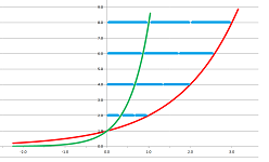
Example. Let's plot $$y=2^{3x}.$$ Once we have, point by point, we realize that it looks very similar to the exponential growth functions we have seen:

A bit of algebra (Rule 3) reveals the connection: $$2^{3x} = (2^{3})^{x} = 8^{x}.$$ It is an exponential function (base $8$)! Therefore, the graph of $y=8^{x}$ is that of $y=2^{x}$ shrunk horizontally by a factor of $3$. $\square$

The lesson is that we can get all exponential functions by stretching and flipping one of them. This fact is demonstrated in the next section.

So, just as we need only one quadratic polynomial, $y=x^2$, we only need one exponential function!

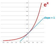
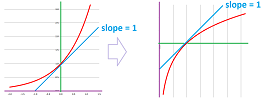
Which one is the one? It is $e^{x}$, the natural base exponent (to be discussed in Chapter 5). It has a special property: it crosses the $y$-axis at $45$ degrees.

It cuts, in a sense, the exponential functions into halves: the “steep” ones and the “shallow” ones.

Example (population growth). Suppose there are $50$ babies born per every $10,000$ of population (Chapter 1). The proportion is: $$ \frac{50}{10000} = 0.005. $$ Therefore, after $x$ years, the population is predicted to become: $$ 1,000,000 \cdot 1.005^{x}. $$ Now, how long will it take for the population to double? We can use trial and error but, generally, we have to solve the equation: $$ 1,000,000 \cdot 1.005^{x}=2,000,000. $$ We will, therefore, need the inverse of the function we just built, presented in the next section. $\square$

The logarithmic function

Example. Bacteria doubles every day. How long does it take to go $8$-fold? Start with function that describes this process and set it equal to $8$: $$ 2^{x} = 8, $$ where $x$ is the time in days. To find this $x$, we'd need the inverse of the exponential function base $2$. $\square$

Since the exponential function is one-to-one and, therefore, invertible with an appropriate choice of range, the following definition is justified.

Definition. For any real $a>0$, the logarithm base $a$ is the inverse of the exponential function base $a$, i.e., $y=a^x$. It is denoted by $$x=\log_a y.$$

Example. Every computed exponent generates a computed logarithm: $$\begin{array}{lll} 2^3=8&\Longrightarrow &\log_2 8=3;\\ 10^2=100 & \Longrightarrow & \log_{10} 100 = 2. \end{array}$$ $\square$

Exercise. What about $\Longleftarrow$?

Just as with the exponential function, in the notation for the logarithm the base is placed below the input of the function: $$\begin{array}{|c|}\hline \quad \text{base}^x\ \text{ vs. }\ \log_\text{base} y. \quad \\ \hline\end{array}$$ The input is a superscript of the base in the former case and the base is a subscript of the input in the latter case.

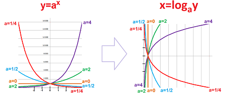
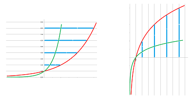
We have acquired, in one stroke, infinitely many new functions. By flipping about the diagonal $y=x$, we have all of their graphs too:

From the basic features of the graph of the exponential function, we derive those for the logarithm; we just interchange $x$ and $y$: $$\begin{array}{l|l} y=a^x & y=\log_a x\\ \hline \text{domain is } (-\infty,+\infty)&\text{range is } (-\infty,+\infty)\\ \text{range is }(0, \infty)& \text{domain is }(0, \infty)\\ y\text{-intercept is }(0, 1)& x\text{ -intercept is }(0, 1)\\ \text{no }x\text{-intercepts}&\text{no }y\text{-intercepts}. \end{array}$$ They are also all one-to-one.

Exercise. Do you see any asymptotes in the graphs?

From the Monotonicity of Exponent theorem in the last section we derive the following about the logarithm.

The statement “$x$ and $y$ increase together” remains true if we interchange $x$ and $y$.

THEOREM (Monotonicity of Logarithm). The logarithm function with base $a > 0$ satisfies the following: $$ \begin{aligned} y=\log_a x & \textrm{ is increasing if } a > 1, \\ y=\log_a x & \textrm{ is decreasing if } a < 1. \end{aligned} $$

Exercise. Prove the theorem.

Now algebra...

The logarithm base $a$ of $y$ is a number! It can be defined verbally as follows:

• $\log_{a} y$ is the power to which you have to raise $a$ to get $y$.

Therefore, we can way that this is the same statement written in two different ways: $$a^x=y\ \text{ vs. }\ \log_a y=x.$$ After all, the relation (Chapter 2) between $x$ and $y$ remains the same.

Example. For a given base, exponents and logarithms come in pairs: $$\begin{array}{lll} a^x=y&\text{means}&\log_a y=x;\\ \hline 2^3=8&\text{means}&\log_2 8=3;\\ 10^2=100 & \text{means }& \log_{10} 100 = 2;\\ 2^{-1}=\frac{1}{2} & \text{means }&\log_{2} \frac{1}{2} = -1;\\ 3^{1/2}=\sqrt{3} & \text{means }&\log_{3}\sqrt{3} = \frac{1}{2}. \end{array}$$ In a sense, every logarithmic expression used to be an exponential expression. This is why, initially, computing logarithms means remembering exponents computed in the past, just like with the roots earlier in this chapter:

• What is $\sqrt[4]{16}$? I seem to recall computing the powers of $2$ and producing $16$ after $4$ steps... So, $\sqrt[4]{16}=2$.
• What is $\log_3 27$? I seem to recall computing the powers of $3$ and producing $27$ after $3$ steps... So, $\log_3 27=3$.

In more complex situations, we have to work our way to a representation of the input of the logarithm as a power of its base.

• What is $\log_{10} .01$? I need to represent $.01$ as a power of $10$... Here it is: $.01=\frac{1}{100}=\frac{1}{10^2}=10^{-2}$. So, $\log_{10} .01 =-2$.
• What is $\log_{4} 2$? I need to represent $2$ as a power of $4$... Here it is: $2=\sqrt{4}=4^{1/2}$. So, $\log_{4} 2=\frac{1}{2}$.

This, however, is hardly a method...

• What is $\log_{4} 5$? I need to represent $5$ as a power of $4$... But it's not... I know! Here it is: $5=4^{\log_4 5}$. So, $\log_{4} 5=\log_{4} 5$!..

This “answer” is just as acceptable as the ones before; we are just unable to simplify this number. $\square$

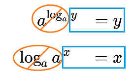
The fact that the exponential function and the logarithm -- of the same base -- are inverses of each other means that they undo each other when composed, in either order. For the pair $$y=a^x \ \text{ and }\ x=\log_a y,$$ we have these two Cancellation Laws: $$\begin{array}{|l|}\hline \quad a^{\log_a y}&=y,\\ \log_a a^x&=x. \quad \\ \hline\end{array}$$

In other words, the outputs of these compositions are the same as the inputs: $$x\to a^x=y\to \log_a y=x;$$ and $$y\to\log_a y=x\to a^x=y.$$ These two flowcharts can be seen in the above formulas, as follows: $$\begin{array}{rrr} 1.&&x\ \\ &&\ (\ x\ )\\ 2.&&{\huge a}\qquad\\ 3.&\log_a(&a^x\qquad&)\\ \end{array}\qquad\qquad\qquad\qquad\begin{array}{rrr} 1.&&&y\\ 2.&&\log_a(&y&)\\ &&{\small \log_a (}&{\small y}&{\small )}\\ 3.&&{\huge a}\qquad \end{array}$$

Warning: the exponent and the logarithm cancel each other only if they are of the same base.

We use these formulas to solve exponential equations.

Example. Solve the following for $x$. $$ 2^{x-5} = 3. $$ To “kill” the exponent and get to $x$, apply its inverse -- to both sides of the equation: the logarithm of the same base: $$ \log_{2} (2^{x - 5}) = \log_{2} (3) .$$ Use the second cancellation law: $$ \begin{array}{ll} x - 5 & = \log_{2} 3, \\ x & = \log_{2} 3 + 5. \end{array} $$ $\square$

Exercise. Solve the equation below. Make up your own equation and solve it. Repeat. $$3^{x^2+1}=2.$$

Exercise. Suppose function $f$ performs the operation: “take the logarithm of”, and function $g$ performs: “take the square root of”. (a) Find the formulas for the two possible compositions. (b) Find their domains.

Algebra of logarithms

Let's go all the way back to the definition of the exponent as repeated multiplication: $$\underbrace{a\cdot a\cdot ... \cdot a}_{x\textrm{ times}}=a^x,$$ for any $x=1,2,3...$. We defined the logarithm of $y$ to be “the power I am to raise $a$ to get $y$”. When $x$ is a natural number, this simply means “the number of times I multiply $a$ by itself to get $y$”: $$\log_a\big( \underbrace{a\cdot a\cdot ... \cdot a}_{x\textrm{ times}} \big)=x.$$

From the Rules of Exponents theorem, we derive the rules about the logarithm. We will continue to use the Cancellation Laws:

We start with the additive rule, Rule 1: $$a^{x+y}=a^x a^y.$$ It comes -- in the case of natural $x$ and $y$ -- from counting two strings of $a$'s: $$a^x\cdot a^y=\overbrace{ \underbrace{a\cdot a\cdot ... \cdot a}_{x\textrm{ times}}\cdot\underbrace{a\cdot a\cdot ... \cdot a}_{y\textrm{ times}} }^{x+y\textrm{ times}}\ =\ \overbrace{ \underbrace{a\cdot a\cdot ... \cdot a}_{a^x}\cdot\underbrace{a\cdot a\cdot ... \cdot a}_{a^y} }^{a^{x+y}}=a^{x+y}.$$ So, we can see that when two numbers are multiplied, the powers, i.e., the logarithms, are added.

THEOREM (Rule 1 of Logarithms). For all $a>0$ and all $X,Y$, we have: $$\log_{a}(XY) = \log_{a} X + \log_{a} Y,$$

Proof. We aim to apply Rule 1 of exponents. But what are those exponents? We define: $$x=\log_{a} X,\ y=\log_{a} Y\ \Longleftrightarrow\ X=a^x,\ Y=a^y.$$ We now apply the logarithm to both sides of Rule 1: $$\begin{array}{rrcrclll} &a^{x+y}&=&a^x& \cdot & a^y\ ,&\text{ apply }\log_a\text{ ... }\\ \Longleftrightarrow &\log_{a} (a^{x+y})&=&\log_{a} (a^x& \cdot & a^y),&\text{ now cancel...}\\ \Longleftrightarrow &x+y&=&\log_{a} (a^x& \cdot &a^y),&\text{ now substitute...}\\ \Longleftrightarrow &\log_{a} X + \log_{a} Y&=&\log_{a} (X& \cdot &Y).& \end{array}$$ $\blacksquare$

Example. In an attempt to “simplify” an expression, we might have to carry out the two following opposite tasks. First, we may have to expand a logarithm into several by reading the formula from left to right: $$\log_2(24)=\log_2(2^3\cdot 3)=\log_2(2^3)+\log_2(3)=3+\log_2 3.$$ Second, we may have to contract several logarithms into one by reading the formula from right to left: $$\log_3(7)+\log_3(2)+1=\log_3(7\cdot 2)+\log_3(3)=\log_3(7\cdot 2\cdot 3)=\log_3(56).$$ The need for one or the other depends on the context or the goal we are pursuing. $\square$

Exercise. Expand the logarithm $\log_3 (24)$. Make your own expression and expand it. Repeat.

Exercise. Contract this to a single logarithm: $\log_2(27)+\log_2(2)+0$. Make your own expression and contract it. Repeat.

Example (tables of logarithms). The logarithms were used for computations in the times before computers. Specifically, Rule 1 was used to multiply large numbers. The key idea is that it converts multiplication to addition, which is easier: $$\begin{array}{ccc} &\log_{a} \big( M& \underbrace{ \times }_{\textrm{multiplication}} &N \big)\\ =& \log_{a} M &\underbrace{+}_{\textrm{addition}} &\log_{a} N. \end{array}$$ They used large tables of pre-computed logarithms and exponents:

To multiply $X$ by $Y$, follow these steps: $$\begin{array}{ll} X\to&\begin{array}{|c|}\hline \text{ table } \\ \hline\end{array}&\to\log X=x\\ &&&\searrow\\ &&&&x+y=z\to&\begin{array}{|c|}\hline \text{ table } \\ \hline\end{array}&\to e^{z}=X\cdot Y,&\text{the end.}\\ &&&\nearrow\\ Y\to&\begin{array}{|c|}\hline \text{ table } \\ \hline\end{array}&\to\log Y=y\\ \end{array}$$ The computation amounts to using the tables three times and doing addition (instead of multiplication) once. $\square$

The two rules -- of exponents and logarithms -- match: $$\begin{array}{cc} a^{x+y}&=&\quad\ a^x\cdot a^y\\ \ \log_{a} X + \log_{a} Y&=&\log_{a}(X\cdot Y). \end{array}$$ In fact, these addition signs on the left and the multiplication signs on the right match up too!

Now the multiplicative rule, Rule 3: $$a^{x y}=(a^x)^y.$$ It comes -- in the case of natural $x$ and $y$ -- from counting repeated strings of $a$'s: $$(a^x)^y=\underbrace{a^x\cdot a^x\cdot ... \cdot a^x}_{y\textrm{ times}}= \left.\begin{array}{lll} a^x\\ a^x\\ ...\\ a^x \end{array}\right\}\ ^{y\text{ times}}=\left.\begin{array}{lll} \underbrace{a\cdot a\cdot ... \cdot a}_{x\textrm{ times}}\\ \underbrace{a\cdot a\cdot ... \cdot a}_{x\textrm{ times}}\\ ...\\ \underbrace{a\cdot a\cdot ... \cdot a}_{x\textrm{ times}}\\ \end{array}\right\}\ ^{y\text{ times}}=\underbrace{a\cdot a\cdot ... \cdot a}_{xy\textrm{ times}}=a^{xy}.$$ So, we can see that when a power is taken to another the power, the former power, i.e., the logarithm, is multiplied by the latter power.

THEOREM (Rule 3 of Logarithms). For all $a>0$ and all $X,y$, we have: $$\log_{a} (X^{y}) = y \log_{a} X .$$

Proof. We aim to apply Rule 3 of exponents. But what is this exponent? We define: $$x=\log_{a} X\ \Longleftrightarrow\ X=a^x.$$ We now apply the logarithm to both sides of Rule 3: $$\begin{array}{rrcrlll} & a^{x y}&=&(a^x)^y,&\text{ apply }\log_a...\\ \Longleftrightarrow &\log_{a} (a^{x\cdot y})&=&\log_{a} \big( (a^x)^y \big),&\text{ now cancel...}\\ \Longleftrightarrow &x\cdot y&=&\log_{a} \big( (a^x)^y \big),&\text{ now substitute...}\\ \Longleftrightarrow &\log_{a} X \cdot y&=&\log_{a} (X^y).& \end{array}$$ $\blacksquare$

Note that choosing $X=a$ in the formula brings us back to the definition: $$\log_{a} (a^{y}) = y \log_{a} a =y.$$

Example. In an attempt to “simplify” an expression, we might have to carry out the two following opposite tasks. First, we may have to expand a logarithm into a multiple of a simpler logarithm by reading the formula from left to right: $$\log_5(32)=\log_5(2^5)=5\log_5 2.$$ Second, we may have to contract a multiple of a logarithm into single one by reading the formula from right to left: $$\frac{1}{2}\log_3 7=\log_3(7^{1/2})=\log_3\sqrt{7}.$$ The need for one or the other depends on the context or the goal we are pursuing. $\square$

Exercise. Expand the logarithm $\log_2 (100)$. Make your own expression and expand it. Repeat.

Exercise. Contract this to a single logarithm: $\frac{1}{3}\log_2(125)$. Make your own expression and contract it. Repeat.

In order to summarize, if

• Rule 1 says that the logarithms turn multiplication into addition, then
• Rule 3 says that the logarithms turn exponentiation into multiplication.

The two main formulas are taken care of, now we consider the conventions about the exponent. They are paired up with facts about the logarithm: $$\begin{array}{r|l} a^0=1&\log_a 1=0\\ a^{-x}=\frac{1}{a^x}& \log_a\frac{1}{Y}=-\log_a Y\\ & \log_a\frac{X}{Y}=\log_a X-\log_a Y\\ \end{array}$$

Example. The last formula can be read from left to right: $$\log_3 6-\log_3 18 =\log_3\frac{6}{18}=\log_3\frac{1}{3}=\log_3 3^{-1}=-1;$$ or from right to left: $$\log_5\frac{1}{25}=\log_5 1-\log_5 25=-2.$$ $\square$

Let's consider again the exponential models (Chapter 1): $$f(x)=Ca^x.$$ Here $x$ is time and $f(x)$ is a quantity that grows or declines with time, in multiples of $a$.

With the help of the logarithm, we are able this time to solve a lot more problems about them. The nature of these problems is “inverse” to those we considered previously. Below we list some familiar models along with old and new problems: $$\begin{array}{l|l|ll} \text{Models}&\text{Direct problems}&\text{Inverse problems}\\ \hline \text{1. Compounded interest:}&\text{Q: How much after 10 years?}&\text{Q: How long to reach }\$ 2000? \\ \$ \text{1000 deposit, 10% APR.}&\text{Substitute: }f(10)=1000\cdot 1.1^{10} &\text{Solve: }1000\cdot 1.1^x=2000\Rightarrow 1.1^x=2.\\ f(x)=1000\cdot 1.1^x&\ \approx \$ 2,593 . &\Rightarrow x=\log_{1.1}2\approx 7.27 \text{ years.}\\ \hline \text{2. Population decline:}&\text{Q: How large after 5 years?}&\text{Q: How long to reach 500K?} \\ \text{1M current, 5% decline.}&\text{Substitute: }f(5)=.95^{5}&\text{Solve: }1\cdot .95^x=.5 \Rightarrow .95^x=.5\\ f(x)=1\cdot .95^x& \ \approx 774K. &\Rightarrow x=\log_{.95}.5\approx 13.51 \text{ years.}\\ \hline \text{3. Radiocarbon decay:}&\text{Q: How much left after 1000 years?}&\text{Q: How long to lose 90%?} \\ \text{5000 years half-life.}&\text{Substitute: }f(5)=.5^{1000/5000}& \text{Solve: } .5^{x/5000}=.1 \Rightarrow x/5000=\log_{.5}.1 \\ f(x)=.5^{x/5000}& \ \approx 87\% . &\Rightarrow x=5000\log_{.5}.1\approx 16610\text{ years.}\\ \hline \end{array}$$ The solutions of the inverse problems are simply applications of the definition of the logarithm!

A different, but related, set of problems is about finding the parameters of the exponential model described indirectly.

Exercise. What APR will double my money in $20$ years?

Exercise. What is the half-life of a radioactive element if an experiment has shown that it loses $.1\%$ of its weight in $1$ year?

Example. Find a representation $y=Ca^{x}$ for this graph:

Pick two points on the graph and use them to write two equations for $f(x) = C a^{x}$:

• $(0, 2)$ is on the graph $\ \Longrightarrow x = 0,\ y = 2\ \Longrightarrow\ Ca^{0} = 2 \Longrightarrow C = 2 $;
• $(2, .25)$ is on the graph $\ \Longrightarrow x = 2,\ y = .25\ \Longrightarrow\ 2a^{2} = .25 \ \Longrightarrow\ a = \sqrt{.125}$.

$\square$

We observed in the last section that we can get all exponential functions by stretching and flipping one of them.

Let's prove this fact. Suppose $a>$ and $b>$ are two bases that we want to match. We use one of the Cancellation Laws and Rule 3 of logarithms: $$y=a^x=b^{\log_b a^x}=b^{(\log_b a)\cdot x}.$$ Therefore, $y=a^x$ is $y=b^x$ shrunk horizontally by a factor of $\log_b a$. We also conclude that $y=\log_a^x$ is $y=\log_b x$ shrunk vertically by a factor of $\log_b a$. Indeed, we have: $$y=\log_a^x=\frac{\log_b x}{\log_b a}.$$

THEOREM (Conversion Formulas). $$\begin{array}{ll} a^x&=b^{(\log_b a)\cdot x}\\ \log_a x&=\frac{\log_b x}{\log_b a}. \end{array}$$

Exercise. Derive the second formula.

So, just as we need only one quadratic polynomial, $y=x^2$, we only need one exponential function. The same applies to the logarithms!

Definition. The logarithm base $e$ is called the natural logarithm and denoted by $y=\ln x$.

Its graph crosses the $y$-axis at $45$ degrees (Chapter 7).

What we discovered is that it suffices to consider a single base -- the standard base -- to get all of the exponential models! Indeed, by making multiples of $y=e^x$, we can get all possible patterns of exponential growth:

Definition. The exponential model is a function: $$y=Ce^{kx},$$ with $k$ called the rate. Furthermore,

• $y=Ce^{kx},\ k>0$, is called the exponential growth model,
• $y=Ce^{kx},\ k<0$, is called the exponential decay model.

Example (population growth). Suppose that the population grows by $10\%$ a year. How long will it take to double? In contrast to the previous analysis of the same problem, we will find the standard, base $e$, exponential model for this setup ($x$ time): $$f(x) = Ce^{kx}, \quad \text{what is }k? $$ Let's assume $f(0) = 1$, then $f(1) = 1.1$. Substitute these into the model: $$\begin{array}{lll} Ce^{k\cdot 0} & = 1 &\Longrightarrow &C = 1; \\ Ce^{k\cdot 1} & = 1.1 &\Longrightarrow &e^{k} = 1.1;\\ &&\Longrightarrow &k= \ln 1.1. \end{array} $$ We have the model: $$f(x)=e^{\ln 1.1\cdot x}.$$ To answer the question we posed, we look for $x$, the time, satisfying: $$\begin{array}{lll} f(x) & = 2, &\text{ substitute...} \\ e^{kx} & = 2, & \text{ solve... } \\ kx & = \ln 2, \\ x &= \frac{\ln 2}{k} &= \frac{\ln 2}{\ln 1.1}\approx 7.27. \end{array} $$ $\square$

Exercise. Is this the same model as the old one, $f(x)=1.1^x$?

Example. Find the inverse of the function: $$y = \frac{e^{x}}{1 + 2e^{x}}.$$ The plan is the same as before: solve the equation for $x$ (while checking that it is one-to-one): $$ \begin{array}{ll} y ( 1 + 2e^{x}) & = e^{x}&\Longrightarrow \\ y + y2e^{x} & = e^{x}&\Longrightarrow \\ 2ye^{x} - e^{x} & = -y &\Longrightarrow \\ (2y - 1 ) e^{x} & = - y&\Longrightarrow \\ e^{x} & = -\frac{y}{2y - 1 }. \end{array}$$ Apply the inverse, which is $\ln$, to both sides of the equation: $$ \underbrace{\ln e^{x}}_{x} = \ln\left(-\frac{y}{2y - 1}\right) \Longrightarrow\ x = \ln\left(-\frac{y}{2y - 1}\right). $$ To find the domain, solve: $$ \left. \begin{array}{ll} 2y - 1 & \neq 0 \\ -\frac{y}{2y - 1} & > 0 \end{array} \right\} \Longrightarrow\ D=(0,1/2).$$ $\square$

Example. Find the inverse of $$ f(x) = e^{x^{3}}.$$ Solve the equation: $y = e^{x^{3}}$, solve for $x$. To get to $x$, we need to get rid of the exponent. To cancel it, apply its inverse to both sides. For $e^{x}$, it's $\ln y$: $$ \begin{array}{ll} \ln y & = \ln e^{x^{3}}, \\ \ln y & = x^{3}. \end{array}$$ Apply the inverse to get to $x$: $$\sqrt[3]{\ln y} = \sqrt[3]{x^{3}} = x.$$ Answer: $ f^{-1}(y) = \sqrt[3]{\ln y} $. $\square$

These are matched up lists of the formulas most frequently used: $$\begin{array}{|l|l|} \hline e^{\ln x}=x&\ln e^x=x\\ e^0=1&\ln 1=0\\ e^xe^y=e^{x+y}&\ln x+\ln y=\ln xy\\ \frac{e^x}{e^y}=e^{x-y}&\ln x-\ln y=\ln \frac{x}{y}\\ \big(e^x\big)^y=e^{xy}& \ln x^y=y\ln x\\ \hline \end{array}$$

The Euclidean plane: distances

In Chapter 2, we introduced the Cartesian coordinate plane as a device for visualizing functions; it's where the graphs live:

We now approach it from another direction: we want to study the Euclidean plane, and Euclidean geometry, algebraically. We superimpose the Cartesian grid over this plane.

The idea of using a coordinate system is to transition

• from geometry: points, then lines, triangles, circles, then planes, cubes, spheres, etc.,
• to algebra: numbers, then combinations of numbers, then functions, etc.

This will allow us to solve geometric problems without measuring. We will initially limit ourselves to the two simplest geometric tasks:

• 1. finding the distance between two points, and
• 2. finding the difference between the directions from a point to other points.

We start with dimension $1$. Let's repeat -- with some minor changes -- the construction from Chapter 1 first.

Suppose we live on a road surrounded by nothingness:

The coordinate system intended to capture what happens on this road is devised to be superimposed on the road.

It is built in several stages:

• 1. a line is drawn, the $x$-axis;
• 2. one of the two directions on the line is chosen as positive, then the other is negative;
• 3. a point $O$ is chosen as the origin;
• 4. a segment of the line -- of length $1$ -- is set as the unit of length;
• 5. the segment is used to measure distances to locations from the origin $O$ -- positive in the positive direction and negative in the negative direction -- and add marks to the line, the coordinates, later the segments are further subdivided to fractions of the unit, etc.

The result is a correspondence: $$\begin{array}{|c|}\hline \quad \text{location } P\ \longleftrightarrow\ \text{ number } x .\quad \\ \hline\end{array}$$ It works in both directions. For example, suppose $P$ is a location on the line. We then find the distance from the origin -- positive in the positive direction and negative in the negative direction -- and the result is the coordinate of $P$, some number $x$. We use the nearest mark to simplify the task.

Conversely, suppose $x$ is a number. We then measure $x$ as the distance to the origin -- positive in the positive direction and negative in the negative direction -- and the result is a location $P$ on the line. We use the nearest mark to simplify the task.

Now that everything is pre-measured we can solve those geometric problems by algebraically manipulating the coordinates of points.

In this section, we consider the first geometric task, distance.

The value of the distance between two locations $P$ and $Q$ is inherited from the Euclidean line that underlines the Cartesian system. It is denoted by $d(P,Q)$. However, how do we express this number in terms of their coordinates, say $x$ and $x'$?

One finds the distance that has been covered on the road by subtracting the number on the milestone in the beginning and the number on the milestone at the end: $$\text{from }P=4 \text{ to } Q=6\ \Longrightarrow\ \text{ distance }=Q-P=6-4=2.$$ But what if we are moving in the opposite direction? The distance should be the same! And the computation should be the same: $$\text{from }Q=6 \text{ to } P=4\ \Longrightarrow\ \text{ distance }=Q-P=6-4=2.$$ In other words, one has to set to subtract the smaller number from the larger one every time in order for the computation to make sense.

THEOREM. The distance between two locations $P$ and $Q$ on the real line given by their coordinates $x$ and $x'$ is

• $d(P,Q)=x'-x$ when $x<x'$,
• $d(P,Q)=x-x'$ when $x>x'$,
• $d(P,Q)=0$ when $x=x'$.

Is there a single formula for this computation? The definition can be seen to be similar to a piece-wise defined function: $$d(P,Q)=\begin{cases} x-x' &\text{ when }x>x',\\ 0 &\text{ when }x=x',\\ x-x' &\text{ when }x<x', \end{cases}=\begin{cases} -(x'-x) &\text{ when }x'-x<0,\\ 0 &\text{ when }x'-x=0,\\ x'-x &\text{ when }x'-x>0. \end{cases}$$ The fact that the distance between two locations is always positive unless the locations coincide suggests a solution.

We have the absolute value function for that: $$|a|=\begin{cases} -a &\text{ when }a<0,\\ 0 &\text{ when }a=0,\\ a &\text{ when }a>0. \end{cases}$$ We just choose $a=x'-x$.

THEOREM (Distance Formula for dimension $1$). The distance between two points on the real line with coordinates $x$ and $x'$ is the absolute values of their difference: $$d(x,x')=|x-x'|=|x'-x|.$$

A frequently used property of the absolute value function is the following.

THEOREM (Triangle Inequality). For any two numbers $x,x'$, we have: $$|x+x'|\le |x|+|x'|.$$

Exercise. Prove the theorem.

The name of the theorem comes from a similar property of the lengths of the sides of a triangle $a,b,c$ (below): $$c<a+b.$$

Exercise. Prove that the point half-way between points $P=x$ and $Q=x'$ -- called their midpoint -- has the coordinate $\frac{x+x'}{2}$.

THEOREM. A linear function stretches the $x$-axis by a factor of $|m|$, where $m$ is its slope.

Proof. This is what happens to the distance between two points $u$ and $v$, which is $|v-u|$, after a linear function $f(x)=mx+b$ with $m$ is applied: $$|f(v)-f(u)|=|(mv+b)-(mu+b)|=|mv-mu|=|m|\cdot |v-u|.$$ The distance has increased by a factor of $m$ (we say that it has decreased by a factor of $m$ when $m<1$). This stretch/shrink factor is the same everywhere. $\blacksquare$

Now the coordinate system for dimension $2$. There is much more going on:

Let's repeat -- with some minor changes -- the construction from Chapter 2 first. Suppose we live on a field with two roads intersecting:

We can then treat either of the two roads as a $1$-dimensional Cartesian system, as above, and use the milestone to navigate. But what about the rest of the field? How do we navigate it? We build a city with a grid of streets:

We also number the streets.

A new coordinate system intended to capture what happens on this city or field is devised to be superimposed on the field. What does it look like?

It is built in several stages:

• 1. two coordinate axes are chosen, the $x$-axis first and the $y$-axis second, with the same units;
• 2. the two axes are put together at their origins so that it is a $90$-degree turn from the positive direction of the $x$-axis to the positive direction of the $y$-axis;
• 3. use the marks on the axes to draw a grid.

We have a correspondence: $$\begin{array}{|c|}\hline \quad \text{location } P\ \longleftrightarrow\ \text{ a pair of numbers } (x,y) ,\quad \\ \hline\end{array}$$ that works in both directions. For example, suppose $P$ is a location on the plane. We then find the distances from either of the two axes to that location -- positive in the positive direction and negative in the negative direction -- and the result is the two coordinates of $P$, some numbers $x$ and $y$. We use the nearest mark to simplify the task.

Conversely, suppose $x$ and $y$ are numbers. First, we measure $x$ as the distance from the $y$-axis -- positive in the positive direction and negative in the negative direction -- and such locations together form a vertical line. Second, we measure $y$ as the distance from the $x$-axis -- positive in the positive direction and negative in the negative direction -- and such locations together form a horizontal line. The intersection of these two lines is a location $P$ on the plane. We use the nearest marks to simplify the task.

The main difference from the $xy$-plane we have seen so far comes from its purpose. In order to do Euclidean geometry on this coordinate plane, squares should be squares and not rectangles, circles should be circles and not ovals, etc.:

Even though we can make larger or smaller plots, the relative dimensions and, consequently, the angles will have to remain the same. To avoid such a disproportional resizing, we need to make sure that we use the same units for $x$- and $y$-axes. This will have to be a square grid.

Example (computers). The $2$-dimensional Cartesian system isn't as widespread as that for dimension $1$. It is however common in a computing environment.

For example, drawing applications allow you to make use of this system -- if you understand it. The location of your mouse is shown in the status bar on the lower left, constantly updated in real time. The main difference is that the origin is in the left upper corner of the image and the $y$-axis is pointing down:

The choice is explained by the way we write: downward.

Similarly, spreadsheet applications use the Cartesian system (also starting at the upper right corner) to provide a convenient way of representing locations of cells:

This idea is instrumental in helping us express a value located in one cell in terms of values located in other cells by making direct or indirect references. For example, this formula computes the square of the number contained in the cell located at the intersection of row $3$ and column $5$: $$\texttt{=R3C5^2}.$$ $\square$

Example. It is entirely possible to have the $x$-axis measured in different units than the $y$-axis. For example, it is typical to measure the distance to the airport in miles but the altitude in feet. For example, one can speak of a point located “$2$ miles east and $5$ kilometers north” from here. However, when this is the case, the geometric formulas above won't be applicable anymore! $\square$

Now that everything is pre-measured, we can solve the geometric problems by algebraically manipulating the coordinates of points.

We turn, again, to the first geometric task, distance.

The value of the distance between two locations $P$ and $Q$ is inherited from the Euclidean plane that underlines the Cartesian system. It is denoted by $d(P,Q)$. However, how do we express this number in terms of their coordinates $(x,y)$ and $(x',y')$? The idea is to use the distance formula from the $1$-dimensional case for either of the two axes!

According to the Distance Formula for dimension $1$, the distance

• between $x$ and $x'$ on the $x$-axis is $|x-x'|$, and
• between $y$ and $y'$ on the $y$-axis is $|y-y'|$.

Then, the segment between the points $P(x,y)$ and $Q=(x',y')$ is the hypotenuse of the right triangle with sides: $|x-x'|$ and $|y-y'|$. Then our conclusion below follows from the Pythagorean Theorem: $$d(P,Q)^2=|x-x'|^2+|y-y'|^2.$$ Since $|a|^2=a^2$ for all $a$, we can remove the absolute value signs.

THEOREM (Distance Formula for dimension $2$). The distance between two points with coordinates $P=(x,y)$ and $Q=(x',y')$ is $$\begin{array}{|c|}\hline \quad d(P,Q)=\sqrt{(x-x')^2+(y-y')^2}. \quad \\ \hline\end{array}$$

The result is so important that one can even say that the $90$ degree angle between the axes was chosen so that we can apply the Pythagorean theorem, again and again.

This is how the two formulas for the two dimensions can be matched up: $$\begin{array}{r|ccc} \text{dimension}&&&x&&y\\ \hline 1&d(P,Q)^2&=&(x-x')^2&\\ 2&d(P,Q)^2&=&(x-x')^2&+&(y-y')^2. \end{array}$$ We will see a continuation of this pattern in Chapter 14.

Here is a familiar property of the lengths of the sides of a triangle $a,b,c$: $$c<a+b.$$

THEOREM (Triangle Inequality). For any three points $P,Q,R$, we have: $$d(P,R)\le d(P,Q)+d(Q,R).$$

Exercise. Derive the theorem from the Distance Formula.

When the triangle degenerates into a segment, we have the triangle inequality for dimension $1$ presented above.

Exercise. Prove that the point $M$ half-way between points $P=(x,y)$ and $Q=(x,y')'$ -- called their midpoint -- is given by their average coordinates: $$M=\left(\frac{x+x'}{2},\frac{y+y'}{2}\right).$$

The simplest geometric figure that relies on the idea of distance is the circle.

Definition. The circle of radius $r>0$ centered at point $P$ on the plane is the set of all points $r$ units away from $P$: $$\{Q:\ d(P,Q)=r\}.$$

In other words, we go from $P$ in all directions for $r$ units and place a point there. Together, they form the circle.

What about its coordinate representation? Suppose $P=(h,k)$. Then, according to the Pythagorean Theorem, or the Distance Formula, any point $Q=(x,y)$ on the circle satisfies the following: $$(x-h)^2+(y-k)^2=d(P,Q)^2=r^2.$$

THEOREM. The circle of radius $r>0$ centered at point $P=(h,k)$ is given by the relation: $$(x-h)^2+(y-k)^2=r^2.$$

In other words, every pair of numbers $x$ and $y$ that satisfy this equation produce a point $(x,y)$ that lies on this circle, and vice versa.

Warning: the center of the circle doesn't belong to the circle.

Exercise. What are the center and the radius of this circle: $x^2+2x+y^2-4y-4=0$? Hint: complete a square.

The following fact will be used numerous times in the future.

Corollary. The circle of radius $r$ centered at the origin is given by: $$\begin{array}{|c|}\hline \quad x^2+y^2=r^2. \quad \\ \hline\end{array}$$

Exercise. Show that every circle of radius $r$ can acquired from the one centered at the origin via shifts.

Exercise. What is the equation of the circle centered at $(1,1)$ and passing through the origin?

Exercise. What is the equation of the circle centered at $(2,1)$ and touching the $y$-axis?

The set of all points that lie inside the circle of radius $r>0$ centered at point $P$ is called an open disk.

THEOREM. The points inside the circle of radius $r>0$ centered at point $P=(h,k)$ satisfy the inequality: $$(x-h)^2+(y-k)^2 < r^2.$$

Exercise. Prove the theorem.

The angles, for both dimensions, are discussed in the end of the chapter.

We postpone the $3$-dimensional case until Chapter 13, but it should be obvious that the construction will start this way:

• 1. build three coordinate axes, etc.

and the correspondence will be:

• location $P\ \longleftrightarrow\ $ a triple of numbers $(x,y,z)$.

One can already see how harder is to visualize things in the $3$-dimensional space, which further justifies the need for the algebraic treatment of geometry that we have presented.

Collectively, these are called $1$-, $2$-, and $3$-dimensional Euclidean spaces.

From geometry to calculus

There are two main entry points to calculus. The first one is via the study of motion. We followed this path in Chapter 1. The second path is via geometry. Starting in this section and then in Chapter 5 and beyond, we will

• compute slopes of curves using differences, and
• compute areas of curved regions using sums.

First, in what direction will light bounce off a curved mirror? We can answer the question if we know the angle of the mirror at every location.

Let's zoom in on the point of contact. We might see a curve made of dots, similar to what we saw in Chapter 1. Every two points give us a line, called the secant line:

Then the slope of the secant line is seen, exactly or approximately, to be the slope of the curve.

Let's review this material. Suppose we have two points on the $xy$-plane: $$(x_1,y_1)\ \text{ and }\ (x_2,y_2).$$ The slope of the line between them is known to be “rise over the run”: $$\text{slope }=\frac{y_2-y_1}{x_2-x_1}.$$

Of course, if we have more points, we have more slopes. Suppose a curve on the $xy$-plane is created by two sequences: $$x_n,\ y_n\ \leadsto\ (x_n,y_n).$$ Knowing all the difference quotients of this pair gives us all the slopes of the curve.

Recall the definition from Chapter 1. Suppose $x_n$ and $y_n$ are two sequences. Then their difference quotient is defined to be the difference of $y_n$ over the difference of $x_n$: $$\frac{\Delta y_n}{\Delta x_n}=\frac{y_{n+1}-y_n}{x_{n+1}-x_n}.$$

Indeed, the numerator, the rise, is the change of $y$, i.e., the difference of $y$: $$\Delta y_n=y_{n+1}-y_n.$$ The denominator, the run, is the change of $x$, i.e., the difference of $x$: $$\Delta x_n=x_{n+1}-x_n.$$

The sequence $x_n$ is often chosen to be an arithmetic progression. In that case, its difference is the increment of the sequence: $$h=\Delta x_n.$$ Then, the difference quotient is simply a multiple of the difference of $y_n$: $$\frac{\Delta y_n}{\Delta x_n}=\frac{y_{n+1}-y_n}{h}=\frac{1}{h}(y_{n+1}-y_n).$$

Example. Consider a parabola, say, $y=f(x)=-(x-1.5)^2+3$. It is plotted, as before, point by point, $y_n=f(x_n)$ with $x_n=.5\cdot n$:

For each two consecutive pair of points, the slope is found by the formula, just as in Chapter 1: $$\texttt{=(RC[-2]-R[-1]C[-2])/(RC[-1]-R[-1]C[-1])}.$$ The line is then drawn via the point-slope formula. $\square$

Exercise. Use the formula above to find and plot the secant lines of the unit circle.

Next, how do we find the area of a curved region?

When we zoom in, we might see that the curve is made of a sequence of points, just as above. The curve on the $xy$-plane is created by two sequences, $(x_n,y_n)$. At its simplest, the region is bound by horizontal edges:

The region is, therefore, made of rectangles! Its area is the width times the height: $\Delta x_n\cdot y_n$. Now, the total area is the sum of the areas of the rectangles; we use the sums just as in Chapter 1: $$A=\sum_{n=1}^{m} \Delta x_n\cdot y_n=h\sum_{n=1}^{m} y_n,$$ when $\Delta x_n=h$.

Example. We know that the area of a circle of radius $r$ is supposed to be $A = \pi r^{2}$. Let's try to confirm this with nothing but a spreadsheet. First, we plot the graph $$y=\sqrt{1-x^2},$$ for various $-1\le x\le 1$. We let the values of $x$ run from $-1$ to $1$ every $.1$ and apply the formula $$\texttt{=SQRT(1-RC[-2]^2)},$$ to get the values of $y$. We the plot these $20$ points; the result is a half-circle:

We next cover, best we can, this half-circle with vertical bars based on the interval $[-1,1]$. We recycle the data: the bases of the bars are our intervals in the $x$-axis and the heights are values of $y$. To see the bars, we simply change the type of the chart plotted by the spreadsheet:

Then the area of the circle is approximated by the sum of the areas of the bars! To let the spreadsheet do all the work, we multiply the heights by the (constant) widths and add up the result in the last column. The last step is to add all entries in this column. We use the formulas for sums just as in Chapter 1: $$\texttt{=R[-1]C+RC[-1]*(RC[-2]-R[-1]C[-2])}.$$ The result is $$\text{Approximate area of the semicircle}= 1.552.$$ It is close to what we know. In summary, the area is the sum of the sequence: $$a_n=\sqrt{1-t_n^2}\cdot .1;$$ i.e., $$A=\sum_{n=1}^{20} .1\cdot\sqrt{1-t_n^2} =\left(\sum_{n=1}^{20}\sqrt{1-t_n^2}\right)\cdot .1.$$ The theoretical result will be proven in Chapter 11. $\square$

Exercise. Use the formula above to find the area under the parabola in the first example.

Trigonometric functions

One encounters numerous examples of repetitive phenomena.

However, very few of the functions introduced so far exhibit this behavior, i.e., are periodic. We introduce a new class of functions.

The trigonometric functions initially come from plane geometry. Suppose we have a right triangle with sides $a,b,c$, with $c$ the longest one facing the right angle.

If $\alpha$ is the angle adjacent to side $a$, then $$\begin{array}{ll} \cos \alpha &=\frac{a}{c};\\ \sin \alpha &=\frac{b}{c};\\ \tan \alpha &=\frac{b}{a}&=\frac{\sin \alpha}{\cos\alpha}. \end{array}$$

We can also think of $\cos \alpha$ as the length of the shadow of the stick of length $1$ turned the angle $\alpha$ in the ground when the sun is above it and $\sin x$ as the length of its shadow on the wall at sunset... Alternatively, the stick is still and it is the sun that is moving:

However, in a triangle, the value of angle $\alpha$ can only be from $0$ to $\pi/2$. This isn't good enough anymore!

This is how we construct $y=\sin (x)$ and $y=\cos (x)$ as functions defined for all values of $x$.

Definition. Suppose a real number $x$ is given. We construct a line segment of length $1$ on the Cartesian plane (with the horizontal axis not marked $x$) starting at $0$ with angle $x$ radians from the horizontal. Then

• the cosine of $x$, denoted by $\cos x$, is the horizontal coordinate of the end of the segment,
• the sine of $x$, denoted by $\sin x$, is the vertical coordinate of the end of the segment.

The domains for $\sin$ and $\cos$ should be the set of all real numbers. But where is it? If the domain isn't the $x$-axis, can we see it elsewhere?

One way to visualize it is to see it on the circle itself. To begin with, the interval $[0,2\pi]$ is wrapped around this circle:

As we shall see in Chapter 13, the radian measure of the angle is equal to the length of the corresponds arc of the unit circle.

Furthermore, keep in mind that $x$ measures the angle but not the angle of any triangle. It is the angle of rotation:

Of course, it can go past $360$ degrees:

That's clockwise, it can also go counterclockwise, with $x$ negative:

The $x$-axis is then seen as a spiral wrapped on this unit circle, like this:

We can now find the values of $y=\sin x$ by examining the values of $x$, as angles, pictured above: $$\begin{array}{l|ccccccc} x&-2\pi&-3\pi/2&-\pi&-\pi/2&0&\pi/2&\pi&3\pi/2&2\pi\\ \hline y&0&1&0&-1&0&1&0&-1&0& \end{array}$$ We can now plot $y=\sin x$ -- point by point following the table above -- with the domain presented as the $x$-axis on the $xy$-plane, as usual:

With more values found, these are the two main trig functions, sine and cosine:

Let's ask and answer some old questions about these new functions.

THEOREM (Periodicity). The functions $\sin$ and $\cos$ are periodic with period $2\pi$, while the function $\tan$ is periodic with period $\pi$; i.e., $$ \begin{aligned} \sin( x + 2 \pi ) & = \sin x, \\ \cos(x + 2\pi) & = \cos x, \\ \tan(x + \pi) & = \tan x, \\ \end{aligned}$$ for all $x$.

THEOREM (Odd-even). The functions $\sin$ and $\tan$ are odd and the function $\cos$ is even.

There are important relations between trigonometric functions.

Suppose we have a right triangle with the hypotenuse (the longest one, facing the right angle) of length $1$.

First, a familiar result is restated.

THEOREM (Pythagorean Theorem). $$\sin^2 x+\cos^2 x=1.$$

Example. When the angle is $45$ degrees, the sine and cosine are equal: $$\sin\frac{\pi}{4}=\cos\frac{\pi}{4}.$$ Therefore, the Pythagorean Theorem implies that $$\sin\frac{\pi}{4}=\cos\frac{\pi}{4}=\frac{\sqrt{2}}{2}.$$ $\square$

Exercise. Find all possible values of $x$ (“pre-image”) for which $$\sin x=\frac{\sqrt{2}}{2}.$$

Exercise. Derive these formulas: $$\begin{array}{ll} \sin \theta &=\pm\frac{\tan \theta}{\sqrt{1 + \tan^2 \theta}};\\ \cos \theta &=\pm\frac{1}{\sqrt{1 + \tan^2 \theta}}. \end{array}$$

Second, for either of the two other angles of the triangle, we have $$\begin{array}{ll} \cos (\text{ angle } )&=\text{ adjacent side };\\ \sin (\text{ angle } )&=\text{ opposite side }. \end{array}$$ If we apply these formulas to either of the angles, we have the following.

THEOREM. $$\sin x =\cos (\pi/2-x)\ \text{ and }\ \cos x=\sin(\pi/2-x).$$

Therefore, the graphs of one function is just a horizontally shifted version of the other. That is why sine and cosine have identical graphs.

Combining the theorem with the periodicity gives us the following.

Corollary. $$\sin x =\cos (x+\pi/2)\ \text{ and }\ \cos x=\sin(x-3\pi/2).$$

Neither function is one-to-one and, therefore, can't have an inverse. However, what we did with $y=x^2$ vs. $x=\sqrt{y}$ can be repeated here:

• restrict the domains of these functions to make them one-to-one.

We choose the branch of $\sin$ over $-\pi/2 \le x \le \pi/2$.

THEOREM. With the domain restricted to $[-\pi/2,\pi/2]$, the sine, $y=\sin (x)$, is a one-to-one function.

Why this interval? Because even restricted $\sin$ remains an odd function and now so is its inverse.

Definition. The arcsine is defined to be the inverse of the sine function restricted to on $[-\pi/2,\pi/2]$, denoted by either: $$\arcsin y=\sin^{-1}y.$$

Thus, we have a pair of inverse functions: $$\begin{array}{ll} y=\sin x,\\ \text{domain } [-\pi/2,\pi/2] \end{array} \quad\text{ and }\quad \begin{array}{ll} x=\sin^{-1}y,\\ \text{domain } [-1,1] \end{array}.$$

The graphs are, of course, the same with just $x$ and $y$ interchanged.

Similarly, we choose the branch of $\cos$ over $0 \le x \le \pi$.

THEOREM. With the domain restricted to $[0,\pi]$, the cosine, $y=\cos (x)$ is a one-to-one function.

Definition. The arccosine is defined to be the inverse of the cosine function on $[0,\pi]$, denoted by either: $$\arccos y=\cos^{-1}y.$$

Thus, we have a pair of inverse functions: $$\begin{array}{ll} y=\cos x,\\ \text{domain } [0,\pi] \end{array} \quad\text{ and }\quad \begin{array}{ll} x=\cos^{-1}y,\\ \text{domain } [-1,1] \end{array}.$$

The tangent function is defined by: $$\tan x =\frac{\sin x}{\cos x}.$$

To find the domain of a fraction, we set the denominator equal to $0$ and solve. Find all $x$'s: $$\cos x = 0 \ \Longrightarrow\ x = ...,\ \frac{\pi}{2},\ \frac{3\pi}{2},\ \frac{5\pi}{2},\ ...$$ Then we should choose the branch of $\tan$ over $-\pi/2< x< \pi/2$.

THEOREM. With the domain restricted to $(-\pi/2,\pi/2)$, the tangent, $y=\tan (x)$, is a one-to-one function.

It's odd and so is its inverse.

Definition. The arctangent is defined to be the inverse of the tangent function restricted to the domain $(-\pi/2,\pi/2)$, denoted by either: $$\arctan y=\tan^{-1}y.$$

Then, we again have a pair of inverse functions: $$\begin{array}{ll} y=\tan x,\\ \text{domain } (-\pi/2,\pi/2) \end{array} \quad\text{ and }\quad \begin{array}{ll} x=\tan^{-1}y,\\ \text{domain } (-\infty,+\infty) \end{array}.$$

We use these functions to solve trigonometric equations.

Example. Solve the following for $x$. $$ \sin (x-5) = .3. $$ To “kill” the sine and get to $x$, apply its inverse -- to both sides of the equation, the arcsine: $$ \arcsin \big(\sin (x - 5) \big) = \arcsin (.3) .$$ We cancel: $$ \begin{array}{ll} x - 5 & = \arcsin .3, \\ x & = \arcsin .3 + 5. \end{array} $$ $\square$

Exercise. Solve the equation below. Make up your own equation and solve it. Repeat. $$\cos^{x^2+1}=.2.$$

Below, we summarize the hypothetical history of appearance of new classes of functions. $$\begin{array}{rrll} \text{ Phenomena: }&&\text{ Classes of functions: }&&\text{ Inverses: }\\ \hline \text{ free fall }\\ &\longrightarrow&\text{ polynomials }\quad&\longrightarrow&\text{ algebraic functions }\\ \hline \text{ gravity }&&\text{ Those functions grow with no bound. }\\ &\longrightarrow&\text{ rational functions }&\\ \hline \text{ population growth/decline, }&&\text{ Those functions are too slow. }\\ \text{ cooling/heating}&\longrightarrow&\text{ exponential functions }\quad&\longrightarrow&\text{ logarithms }\\ \hline \text{ waves, planetary motion }&&\text{ Those functions aren't periodic. }\\ &\longrightarrow&\text{ trig functions }\quad&\longrightarrow&\text{ inverse trig functions}\\ \hline \text { new phenomena }&&\text{ Those functions don't conform.}\\ &\longrightarrow&\text{ abstract functions} \end{array}$$

Exercise. What are the inverses of the rational functions?

The Euclidean plane: angles

In this section we take up the second geometric task, directions, in the Euclidean space equipped with the Cartesian coordinate system.

First, the $1$-dimensional Euclidean space, i.e., just the $x$-axis.

What does a direction on the real line mean? We will pursue the following approach.

Definition. If a line segment's starting point is the origin, i.e., it's $OP$, it is called a ($1$-dimensional) vector.

There are exactly two directions for a vector: positive and negative. In addition to a direction, a vector has its magnitude, which is the absolute value of the coordinate of its terminal point. It is denoted by: $$||OP||=|P|.$$

How do we compare the directions from the origin $O$ toward locations $P$ and $Q$ ($P\ne O,\ Q\ne O$)? There can be only two possibilities:

• if $P$ and $Q$ are on the same side of $O$ then the directions are the same,
• if $P$ and $Q$ are on the opposite sides of $O$ then the directions are the opposite.

When the vectors are represented by their coordinates, $x$ and $x'$, the analysis of directions becomes algebraic:

• if $x>0,\ x'>0$ or $x<0,\ x'<0$ then the directions are the same,
• if $x>0,\ x'<0$ or $x<0,\ x'>0$ then the directions are the opposite.

Fortunately, the product provides us with a single expression that makes this determination.

THEOREM (Directions for dimension $1$). The directions from $0$ to $x\ne 0$ and $x'\ne 0$ are

• the same if and only if $x\cdot x'>0$; and
• the opposite if and only if $x\cdot x'<0$.

Exercise. Restate the theorem in terms of $\operatorname{sign}(x)$. Explain the case: $x=0$ or $x'=0$.

This brings us to the idea of an oriented interval, or segment, within the axis. Any two distinct points $P$ and $Q$ produce two intervals: $PQ$ and $QP$. These two intervals have opposite directions and we say that they have opposite orientations. Furthermore, since the direction of the $x$-axis is set ahead of time, we can match the direction of the interval with it, as follows.

Definition.

• If $P<Q$, the segment $PQ$ is called positively oriented and
• if $P>Q$, the segment $PQ$ is called negatively oriented.

In fact, we adopt the following convention: $$QP=-PQ.$$ So, a ruler has two ends and there are two ways to place it along a measuring tape...

Second, the $2$-dimensional Euclidean space, i.e., the $xy$-plane.

The value of the angle between two directions, i.e., the lines, from $O$, to $P$ and to $Q$, is inherited from the Euclidean plane that underlines the Cartesian system. It is denoted by $\widehat{QOP}$. However, how do we express this number in terms of their coordinates $P=(x,y)$ and $Q=(x',y')$?

Let's first consider a special case: $Q=(1,0)$. The question becomes that about the angle the line $OP$ with the $x$-axis. It is determined from the coordinates of $P=(x,y)$ via simple trigonometry.

Exercise. Explain these computations.

One of these formulas is especially important.

THEOREM (Slope). The tangent of the angle $\alpha$ between the $x$-axis and the line from $O$ to $P=(x,y)\ne O$ is equal to the slope of this line: $$\tan \alpha =\frac{y}{x}.$$

We will rely on the following fact in the future.

Corollary. The tangent of the angle $\alpha$ between the $x$-axis and the line from $Q=(x_0,0)$, the $x$-intercept, to $P=(x,y)\ne Q$ is equal to the slope of this line: $$\tan \alpha =\frac{y}{x-x_0}.$$

Recall from Euclidean geometry that two line are called parallel if they form the same angle with a given line.

As this line can be chosen to be the $x$-axis, we deal with the angle $\alpha$ above, and its tangent, and, therefore, the slope of the line. We conclude the following.

THEOREM (Parallel lines). Two (non-vertical) lines on the $xy$-plane are parallel if and only if they have equal slopes.

The statement can be abbreviated as follows: $$y=mx+b \ || \ y=m'x+b' \ \Longleftrightarrow\ m=m'.$$

Exercise. Find the line parallel to $y=-3x$ that passes through the point $(1,1)$. Suggest another line and repeat.

The case not covered by the theorem is a pair of two vertical lines. However, we know that they are all parallel to each other and not parallel other lines. We, therefore, we have answered the question about parallelism.

Lines on the plane are its subsets. It is, therefore, natural to ask about their intersection. We know from Euclidean geometry that two parallel lines don't intersect. If they did, they'd form a triangle with the sum of the angles above $180$ degrees:

We can now prove this fact algebraically.

Corollary. Parallel lines don't intersect. Conversely, non-parallel lines intersect.

Proof. According to the last theorem, we have two lines with the same slope, $m$, and two different $y$-intercepts, $b$ and $c$: $$\begin{cases} y&=&mx&+b ,\\ y&=&mx&+c . \end{cases}$$ It's a system of linear equations! Subtracting the two equations produces: $b-c=0$. There is no solution and, therefore, no intersection. $\blacksquare$

Exercise. Prove the converse part of the corollary.

Exercise. Prove that vertical lines don't intersect each other and do intersect all other lines.

Example (mixtures). Recall an example from Chapter 2: is it possible to create, from the Kenyan coffee - $\$2$ per pound -- and the Colombian coffee - $\$3$ per pound, $6$ pounds of blend with the total price of $\$14$? The problem is solved via a system of linear equations: $$\begin{cases} x&+y &= 6 ,\\ 2x&+3y &= 14. \end{cases}$$ Without even solving it, we follow this line of thought:

• the slopes of the two lines are different; therefore,
• the lines are not parallel; therefore,
• the lines intersect; therefore,
• the system has a solution.

So, it is possible to create such a blend! It would be impossible if both types of coffee were priced at $\$2$ per pound. $\square$

Exercise. Justify the last statement (second option) using the theorem about parallel lines. What is the third option?

We now consider the general case of an angle between two lines. The geometry is illustrated below:

We have the following for the two angles from the $x$-axis to $P=(x,y)$ and to $Q=(x',y')$ respectively: $$\begin{array}{lll} \cos \alpha =\frac{x}{\sqrt{x^2+y^2}},& \cos \beta =\frac{x'}{\sqrt{{x'}^2+{y'}^2}};\\ \sin \alpha =\frac{y}{\sqrt{x^2+y^2}},& \sin \beta =\frac{y'}{\sqrt{{x'}^2+{y'}^2}}. \end{array}$$ The formulas look complicated but keep in mind that the denominators are just the distances from $O$ to $P$ and $Q$ respectively.

However, our interest isn't these two angles but their difference, $$\widehat{QOP}=\alpha - \beta.$$ Fortunately, there is another trigonometric formula that allows us to represent the cosine of this angle in term of the four values above: $$\begin{array}{lll} \cos(\alpha - \beta) &= \cos \alpha \cos \beta + \sin \alpha \sin \beta\ \\ &=\frac{x}{\sqrt{x^2+y^2}}\frac{x'}{\sqrt{{x'}^2+{y'}^2}}+\frac{y}{\sqrt{x^2+y^2}}\frac{y'}{\sqrt{{x'}^2+{y'}^2}}&\text{ ...we substitute}\\ &=\frac{xx'+yy'}{\sqrt{x^2+y^2}\sqrt{{x'}^2+{y'}^2}}&\text{ ...and simplify}. \end{array}$$ The two parts of the denominator are the distances to $P=(x,y)$ and $Q=(x',y')$: $$d(O,P)=\sqrt{x^2+y^2},\quad d(O,Q)=\sqrt{{x'}^2+{y'}^2}.$$ But what about the numerator?

This formula can be simplified by applying the following idea.

Definition. If a segment's starting point is the origin, i.e., it's $OP$, it is called a ($2$-dimensional) vector. Its components are the coordinates of its terminal point, according to the following notation: $$\begin{array}{|c|}\hline \quad P=(a,b)\ \Longleftrightarrow\ OP=<a,b>. \quad \\ \hline\end{array}$$

A vector has a direction, the direction of the line, and a magnitude, defined as follows.

Definition. The magnitude of a vector $OP=<a,b>$ is defined to be the distance from $O$ to its tip $P$: $$||<a,b>||=\sqrt{a^2+b^2}.$$

Then the formula above is rewritten as follows: $$\cos(\alpha - \beta) =\frac{xx'+yy'}{||<x,y>||\cdot ||<x',y'>||}.$$

We now would like to make sense of the numerator of this fraction.

Definition. The dot product of two vectors $<a,b>$ and $<c,d>$ is defined to be: $$<a,b>\cdot <c,d>=ac+bd.$$

Warning: the meaning of the dot “$\cdot$” is determined by the context.

The dot product is connected back to the magnitude by the formula: $$||<a,b>||^2=<a,b>\cdot <a,b>.$$

The formula for the angle we are developing takes a simpler form now: $$\cos(\alpha - \beta) =\frac{<x,y>\cdot <x',y'>}{||<x,y>||\, ||<x',y'>||}.$$ We conclude the following.

THEOREM (Directions for dimension $2$). The angle between the vectors $OP$ and $OQ$, where $P=(x,y)\ne O$ and $Q=(x',y')\ne O$, is determined by: $$\cos \widehat{QOP}=\frac{<x,y>\cdot <x',y'>}{||<x,y>||\, ||<x',y'>||}.$$

Exercise. Explain the difference between “the angle between two vectors” and “the angle between two lines”.

Exercise. What is the angle between the lines $y=-2x+3$ and $y=x-1$? Suggest another pair of lines and repeat.

Exercise. Find a line that makes a $30$ degree angle with the line $y=-2x+3$? Suggest another angle and another line and repeat.

Exercise. Derive a formula for the sine of this angle.

Example. When these vectors are equal to each other, we have: $$\cos \widehat{POP}=\frac{<x,y>\cdot <x,y>}{||<x,y>||\, ||<x,y>||}=\frac{||<x,y>||^2}{||<x,y>||^2}=1.$$ Therefore, $\widehat{POP}=0$, as expected. $\square$

Example. When the terminal point of both vectors lie on the $x$-axis, i.e., $y=y'=0$, the formula turns into the following: $$\cos \widehat{QOP}=\frac{xx'}{|x|\,|x'|}=\frac{x}{|x|}\frac{x'}{|x'|}=\operatorname{sign}(x)\cdot \operatorname{sign}(x').$$ There are only two possibilities here, $1$ or $-1$, and, therefore, $\widehat{QOP}$ can only be either $0$ or $180$ degrees. $\square$

Exercise. Show how this fact demonstrates the theorem about the directions in dimension $1$.

A case of an especial importance is, when are two vectors or two lines perpendicular? The example of these two lines: $y=2x$ and $y=-\frac{1}{2}x$, suggests that the slopes will have to be negative reciprocals of each other:

Let's prove this fact using the theorem. We have: $$0=\cos \pi/2=\frac{<x,y>\cdot <x',y'>}{||<x,y>||\,||<x',y'>||}.$$ Therefore, $$<x,y>\cdot <x',y'>=0\ \Longleftrightarrow\ xx'+yy'=0\ \Longleftrightarrow\ xx'=-yy'\ \Longleftrightarrow\ \frac{y}{x}\cdot \frac{y'}{x'}=-1.$$ But these two expressions are the slopes of the lines!

THEOREM (Perpendicular lines). Two lines with slopes $m$ and $m'$ are perpendicular if and only if $mm'=-1$.

Since any vertical line is perpendicular to any horizontal line and vice versa, we have solved the problem of perpendicularity. This is the summary:

Exercise. Find the line perpendicular to $y=-3x$ that passes through the point $(1,1)$. Suggest another line and repeat.

The theory of vectors is further developed in Chapter 16.

The axes contain oriented segments. These segments then form oriented rectangles in the plane.

The ones above are all positively oriented, but, for example, combining a positively oriented segment and a negatively oriented segment will produce a negatively oriented rectangle:

So, since a piece of fabric has two sides, inside and outside, it can be placed on the table in two ways... This idea is further developed in Chapter 20.

Solving inequalities

As explained in Chapter 2, to solve an inequality with respect to $x$ means the same as solving an equation -- to find all values of $x$ that, when substituted, produce a true statement. For example, consider how this inequality is solved: $$x+2\ge 5\ \Longrightarrow\ x\ge 3.$$ This is an abbreviated version of the following statement:

• if $x$ satisfies the inequality $x+2\ge 5$ then $x$ satisfies the inequality $x\ge 3$.

Plug in some and see if they check out: $$\begin{array}{ll} x= 0&(0)+2= 2\not\ge 5&\text{No!}\\ x= 1&(1)+2= 3\not\ge 5&\text{No!}\\ x= 2&(2)+2= 4\not\ge 5&\text{No!}\\ x= 3&(3)+2= 5\ge 5&\text{Yes!}\\ x= 4&(4)+2= 6\ge 5&\text{Yes!}\\ \end{array}$$ Of course, this trail-and-error method is unfeasible because there are infinitely many possibilities.

A method of how we may arrive to the answer is discussed in this section. The analysis follows that for solving equations presented in Chapter 3.

We will address a simple kind of inequality:

• $x$ is present only once, in the left-hand side.

For example, we might have: $$5\cdot\Big( \left( \frac{x}{2}+1\right)^2+3 \Big)-17\ge 3.$$ Many inequalities can be reduced to this kind via algebraic manipulations; for example, $$2x+2\ge 5+x\ \Longrightarrow\ x+2\ge 5.$$

Starting with such an inequality, our goal is -- through a series of manipulations -- to arrive to an inequality with an isolated $x$, i.e., only $x$ on the left and no $x$ on the right, like this: $$x\ge \sqrt{17}.$$

Warning: this is an inequality.

What we see above is a single $x$ “wrapped” in several layers of functions, i.e., a composition of several functions applied to $x$. We will remove these layers one by one, from the outside in.

Warning: this plan does not work for many familiar types of inequalities including quadratic inequalities.

The main idea is the same as for equations:

• we apply a function to both sides of the inequality producing a new inequality.

For example, if we have an inequality, say, $$x+2\ge 5,$$ we treat the two sides of the inequalities as two values of the same variable, say, $y$. If we add $2$ to both, the relation between them remains. More precisely, we have: $$x+2\ge 5,\ \text{ apply }z= y-2\ \Longrightarrow\ (x+2)-2\ge 3-2\ \Longrightarrow\ x\ge 3.$$ We produce -- from an inequality satisfied by $x$ -- another inequality satisfied by $x$.

However, the challenge is that any increasing function applied this way will produce a new, correct, inequality! $$\begin{array}{lll} x+2\ge 5,& \text{apply }z= y+2& \Longrightarrow\ (x+2)+2\ge 5+2& \Longrightarrow\ x+4\ge 7;\\ x+2\ge 5,& \text{apply }z= 7y& \Longrightarrow\ 7\cdot (x+2)\ge 7\cdot 5;\\ x+2\ge 5,& \text{apply }z= y^3& \Longrightarrow\ (x+2)^3\ge 5^3. \end{array}$$ Indeed, it is the definition of an increasing function: larger inputs (an inequality) produce -- under $g$ -- larger outputs (another inequality), always: $$\newcommand{\ra}[1]{\!\!\!\!\!\xrightarrow{\quad#1\quad}\!\!\!\!\!} \newcommand{\la}[1]{\!\!\!\!\!\xleftarrow{\quad#1\quad}\!\!\!\!\!} \newcommand{\da}[1]{\left\downarrow{\scriptstyle#1}\vphantom{\displaystyle\int_0^1}\right.} \newcommand{\ua}[1]{\left\uparrow{\scriptstyle#1}\vphantom{\displaystyle\int_0^1}\right.} \begin{array}{ccc} \text{old inequality:}&a& \ge &b\\ g\nearrow&\da{g}& &\da{g}\\ \text{new inequality:}&g(a) & \ge &g(b) \end{array}\qquad\qquad\begin{array}{ccc} \text{old inequality:}&a& \ge &b\\ g\searrow&\da{g}& &\da{g}\\ \text{new inequality:}&g(a) & \le &g(b) \end{array}$$ So, we have, for any increasing function $g$: $$x+2\ge 5\ \Longrightarrow\ g(x+2)\ge g(5).$$ The opposite is true for any decreasing function $g$: $$x+2\ge 5\ \Longrightarrow\ g(x+2)\le g(5).$$

There are infinitely many possibilities for this function $g$: $$\begin{array}{rrcll} x+4\ge 7 & & 7\cdot (x+2)\ge 7\cdot 5 & & (-2)\cdot (x+2)\le (-2)\cdot 5\\ & \nwarrow & \uparrow & \nearrow\\ x+5\ge 8 & \leftarrow & \begin{array}{|c|}\hline \quad x+2\ge 5 \quad \\ \hline\end{array} & \to & 2^{x+2}\ge 2^5\\ & \swarrow & \downarrow & \searrow\\ x+6\ge 9 & & (x+2)^3\ge 5^3 & & \sqrt{x+2}\ge \sqrt{5}\\ \end{array}$$ If $x$ satisfies the inequality in the middle, it also satisfies the rest of the inequalities. If we want to solve the original inequality, we will need a foresight to choose a function to apply that will make the inequality simpler. Just as with equations, if between us and $x$ there is a function, we remove it by applying its inverse to the inequality.

Example. What if we have several functions applied consecutively to $x$? Which function do we choose to apply? In the inequality, $$5\cdot\Big( \left( \frac{x}{2}+1\right)^2+3 \Big)-17\ge 3,$$ the last operation on the left is $-17$. That's the function we face and the inverse of this function is to be applied. We choose: $$f(z)= z-17,$$ where $$z= 5\cdot\Big( \left( \frac{x}{2}+1\right)^2+3 \Big).$$ Then we apply $$f^{-1}(y)= y+17.$$ to both sides. We conclude: $$z-17\ge 3\ \Longrightarrow\ (z-17)+17\ge 3+17\ \Longrightarrow\ z\ge 20.$$ We have a new inequality now: $$5\cdot\Big( \left( \frac{x}{2}+1\right)^2+3 \Big)\ge 20.$$ As we progress, we apply the inverse of the function that appear first in the inequality. We have the following sequence of steps “unwrapping” the parentheses one pair at a time: $$\begin{array}{lclc} 5\cdot\Big( \left( \frac{x}{2}+1\right)^2+3 \Big)\ge 20& \Longrightarrow&5\cdot\Big( \left( \frac{x}{2}+1\right)^2+3 \Big)/5\ge 20 /5&\Longrightarrow&\\ \left( \frac{x}{2}+1\right)^2+3 \ge 4 &\Longrightarrow&\left( \frac{x}{2}+1\right)^2+3-3 \ge 4-3 &\Longrightarrow&\\ \left( \frac{x}{2}+1\right)^2 \ge 1 &\Longrightarrow&\sqrt{\left( \frac{x}{2}+1\right)^2} \ge \sqrt{1} &&\\ \end{array}$$ The last inequality produces two cases: $$\begin{array}{rcl} &\sqrt{\left( \frac{x}{2}+1\right)^2} \ge \sqrt{1}\\ \swarrow&&\searrow\\ \end{array}$$ $$\begin{array}{lll|c|ll} z= \frac{x}{2}+1\ge 0&&&\texttt{ OR }&z= \frac{x}{2}+1\le 0\\ \hline \left( \frac{x}{2}+1\right)^2 &\ge 1 &\Longrightarrow&\texttt{ OR }&-\left( \frac{x}{2}+1\right)^2 &\ge 1 &\Longrightarrow&\\ \frac{x}{2}+1 &\ge 1 &\Longrightarrow&\texttt{ OR }&\frac{x}{2}+1 &\le -1 &\Longrightarrow \\ \frac{x}{2} &\ge 0 &\Longrightarrow&\texttt{ OR }&\frac{x}{2} &\le -2 &\Longrightarrow&\\ x &\ge 0&&\texttt{ OR }&x&\le -4. \\ \end{array}$$ The values that satisfy either $x\ge 1$ or $x\le -4$ satisfy their respective conditions. Therefore, the solution set is $(-\infty,-4]\cup [0,+\infty)$. $\square$

Exercise. Solve the inequality: $$5\cdot\Big( \left( \frac{x^2}{2}+1\right)^2+3 \Big)-17\ge 3.$$

Exercise. Solve the inequality: $$\left( 5\cdot\Big( \left( \frac{x}{2}+1\right)^2+3 \Big)-17\right)^3\ge 27.$$ Make up your own inequality and solve it. Repeat.

Using invertible functions ensures that we will have the same solution set as we progress through the stages. For example, this is how we would rather present the solution of the very first inequality in this section: $$x+2\ge 5\ \Longleftrightarrow\ x\ge 3.$$ This is an abbreviated version of the following statement:

• $x$ satisfies $x+2\ge 5$ if and only if $x$ satisfies $x\ge 3$.

Repeated as many times as necessary, the solution set of each inequality is the same as that of the original inequality!

Example. Two complete solutions are below: $$\begin{array}{lll} 2(x+2)-3\ge 5x\ \Longleftrightarrow\ 2x+4-3\ge 5x\ \Longleftrightarrow\ -3x\ge -1\ \Longleftrightarrow\ x\le 1/3;\\ x^2+1\ge 0\ \Longleftrightarrow\ x^2\ge -1\ \Longleftrightarrow\ {\bf R}. \end{array}$$ $\square$

So, to solve the type of inequality we face -- a variable $x$ subjected to a sequence of functions -- we apply the inverses of these functions in the reversed order. We may have to split the domain of the function so that it is one-to-one on each of the subsets. As we have seen, this step also splits our inequality.

Example. A solution is below: $$\begin{array}{lll} x^2\ge 1\ \Longleftrightarrow\ x\le -1\ \texttt{ OR }\ x\ge 1. \end{array}$$ $\square$

Exercise. Solve the inequality in this manner: $$2^{x+1}\ge 3.$$

Exercise. Solve the inequality in this manner: $$2^{x^2+1}\ge 3.$$ Make up your own inequality and solve it. Repeat.

Example. If we, instead of a single $x$, face an expression that depends on $x$, we treat it as just another variable: $$5\cdot\Big( \left( x^2+x+1\right)^2+3 \Big)-17\ge 3\ \Longrightarrow \ \text{ choose }\ y= x^2+x+1$.$$ We substitute: $$5\cdot\Big( (y)^2+3 \Big)-17\ge 3,$$ and go after $y$ by following the same plan as before. Once this inequality is solved, you have a much simpler inequality, or inequalities, for $x$: $$x^2+x+1 \ge 1\ \texttt{ OR }\ x^2+x+1\le -4.$$ $\square$

Exercise. Finish the solution. Make up your own inequality and solve it. Repeat.

Example. Another solution is below: $$\begin{array}{lll} \sqrt{x^2-3x+2}\ge 0\ \Longleftrightarrow\ \sqrt{y}\ge 0\ \texttt{ AND }\ y= x^2-3x+2\\ \Longleftrightarrow\ y\ge 0\ \Longleftrightarrow\ x^2-3x+2\ge 0\ \Longleftrightarrow\ x\ge 2\ \texttt{ OR }\ x\le 1\\ \Longleftrightarrow\ (-\infty,1]\cup [2,+\infty). \end{array}$$ $\square$