Vector and complex variables

Where do matrices come from?

Matrices appear in systems of linear equations.

Problem 1. Suppose we have coffee that costs $\$3$ per pound. How much do we get for $\$60$?

Solution: $$3x=60\ \Longrightarrow\ x=\frac{60}{3}.$$

Problem 2. Given: Kenyan coffee - $\$2$ per pound, Colombian coffee - $\$3$ per pound. How much of each do you need to have $6$ pounds of blend with the total price of $\$14$?

The setup is the following. Let $x$ be the weight of the Kenyan coffee and let $y$ be the weight of Colombian coffee. Then the total price of the blend is $\$ 14$. Therefore, we have a system: $$\begin{cases} x&+&y &= 6 \\ 2x&+&3y &= 14 \end{cases}.$$

Solution: From the first equation, we derive: $y=6-x$. Then substitute into the second equation: $2x+3(6-x)=14$. Solve the new equation: $-x=-4$, or $x=4$. Substitute this back into the first equation: $(4)+y=6$, then $y=2$.

But it was so much simpler for Problem 1! How can we mimic this equation and get a single equation for the system in Problem 2? What if we think of the former problem as if it is about a blend of one ingredient? This is how progress: $$\begin{array}{l|cc} &\text{ Problem 1 }&\text{ Problem 2 }\\ \hline \text{the unknown }&x&X=<x,y>\\ \text{the coefficient }&3&?\\ \text{the product }&60&?\\ \end{array}$$ We transition to from numbers to vectors. But what are the operations?

Let's collect the data in the equation in these tables: $$\begin{array}{|ccc|} \hline 1\cdot x&+1\cdot y &= 6 \\ \hline 2\cdot x&+3\cdot y &= 14\\ \hline \end{array}\leadsto \begin{array}{|c|c|c|c|c|c|c|} \hline 1&\cdot& x&+&1&\cdot& y &=& 6 \\ 2&\cdot& x&+&3&\cdot&y &=& 14\\ \hline \end{array}\leadsto \begin{array}{|c|c|c|c|c|c|c|} \hline 1& & & &1& & & & 6 \\ &\cdot& x&+& &\cdot& y &=& \\ 2& & & &3& & & & 14\\ \hline \end{array}$$ We see tables starting to appear... We call these tables matrices.

The four coefficients of $x,y$ form the first table: $$A = \left[\begin{array}{} 1 & 1 \\ 2 & 3 \end{array}\right].$$ It has two rows and two columns. In other words, this is a $2 \times 2$ matrix.

The second table is on the right; it consists of the two “free” terms (free of $x$'s and $y$'s) in the right hand side: $$B = \left[\begin{array}{} 6 \\ 14 \end{array}\right].$$ This is a $2$-dimensional vector.

The third table is less visible; it is made of the two unknowns: $$X = \left[\begin{array}{} x \\ y \end{array}\right].$$ This is also a $2$-dimensional vector.

The following combination of $A$ and $B$ is called the augmented matrix of the system: $$[A|B]= \left[\begin{array}{ll|l} 1 & 1 &6\\ 2 & 3 &14 \end{array}\right].$$ It's an abbreviation.

Is there more to this than just abbreviations? How does this matrix interpretation of the system help? Both $X$ and $B$ are column-vectors in dimension $2$ and matrix $A$ makes the latter from the former. This is very similar to multiplication of numbers; after all they are vectors of dimension $1$... Let's match the two problems and their solutions: $$\begin{array}{ccc} \dim 1:&a\cdot x=b& \Longrightarrow & x = \frac{b}{a}& \text{ provided } a \ne 0,\\ \dim 2:&A\cdot X=B& \Longrightarrow & X = \frac{B}{A}& \text{ provided } A \ne 0, \end{array}$$ Now if we can just make sense of the new algebra...

Here $AX=B$ is a matrix equation and it's supposed to capture the system of equations in Problem 2. Let's compare the original system of equations to $AX=B$: $$\begin{array}{} x&+y &= 6 \\ 2x&+3y &=14 \end{array}\ \leadsto\ \left[ \begin{array}{} 1 & 1 \\ 2 & 3 \end{array} \right] \cdot \left[ \begin{array}{} x \\ y \end{array} \right] = \left[ \begin{array}{} 6 \\ 14 \end{array} \right].$$ We can see these equations in the matrices. First: $$1 \cdot x + 1 \cdot y = 6\ \leadsto\left[ \begin{array}{} 1 & 1 \end{array} \right] \cdot\left[ \begin{array}{} x \\ y \end{array} \right] = \left[ \begin{array}{} 6 \end{array} \right].$$ Second: $$3x+5y=35\ \leadsto\ \left[ \begin{array}{} 2 & 3 \end{array} \right] \cdot \left[ \begin{array}{} x \\ y \end{array} \right] = \left[ \begin{array}{} 14 \end{array} \right].$$ This suggests what the meaning of $AX$ should be. We “multiply” either row in $A$, as a vector, by the vector $X$ -- via the dot product!

Definition. The product $AX$ of a matrix $A$ and a vector $X$ is defined to be the following vector: $$A=\left[ \begin{array}{} a & b \\ c & d \end{array} \right],\ X=\left[ \begin{array}{} x \\ y \end{array} \right]\ \Longrightarrow\ AX=\left[ \begin{array}{} a & b \\ c & d \end{array} \right] \cdot \left[ \begin{array}{} x \\ y \end{array} \right]=\left[ \begin{array}{} ax+by \\ cx+dy \end{array} \right].$$

Before we study matrices as functions in the next section, let's see what insight our new approach provides for our original problem...

The solution considered initially has the following geometric meaning. We can think of the two equations as equations about the coordinates of points, $(x,y)$, in the plane: $$\begin{array}{ll} x&+y &= 6 ,\\ 2x&+3y &= 14. \end{array}$$ In fact, either equation is a representations of a line on the plane. Then the solution $(x,y)=(4,2)$ is the point of their intersection:

The new point of view is very different: instead of the locations, we are after the directions.

We can think of the two equations as equations about the coefficients, $x$ and $y$, of vectors in the plane: $$x\left[\begin{array}{c}1\\2\end{array}\right]+y\left[\begin{array}{c}1\\3\end{array}\right]=\left[\begin{array}{c}6\\14\end{array}\right].$$ In other words, we need to find a way to stretch these two vectors so that the resulting combination is the vector on the right:

Example. What if the blend to contain another, third, type of coffee? Given three prices per pound: $2,3,5$. How much of each do you need to have $6$ pounds of blend with the total price of $14$?

Let $x$, $y$, and $z$ be the weights of the three types of coffee respectively. Then the total price of the blend is $14$. Therefore, we have a system: $$\begin{cases} x &+ &y &+& z &= 6 \\ 2x &+ &3y &+& 5z &= 14 \end{cases}.$$ We know that these equations represent two planes in ${\bf R}^3$. The solution is then their intersection:

There are, of course, infinitely many solutions. An additional restriction in the form of another linear equation may reduce the number to one... or none. The variety of possible outcomes is by far higher than in the $2$-dimensional case; they are not discussed in this chapter.

The algebra, however, is the same! The three prices per pound can be written in a vector, $<2,3,5>$, and the first equation becomes the dot product: $$<2,3,5>\cdot <x,y,z>=6.$$ And the whole system can be written in the form of exactly the same matrix equation: $$AX=B.$$ This equation will re-appear no matter what number of variables, $m$, we have or the number of equations, $n$; we will have an $n\times m$ matrix: $$\begin{array}{ll}\begin{array}{lllllllll} && 1 & 2 & 3 & ... & m \end{array}\\ \begin{array}{c} 1 \\ 2 \\ \vdots\\ n \end{array} \left[\begin{array}{rrrrrrrrrrrr} 2 & 0 & 3 &... & 2 \\ 0 & 6 & 2 &... & 0 \\ \vdots & \vdots & \vdots &... &\vdots \\ 3 & 1 & 0 &... & 12 \end{array}\right]\end{array}. $$ $\square$

Warning: What is the difference between tables of numbers and matrices? The algebraic operations discussed here.

Transformations of the plane

We saw in Chapter 18 real-valued functions of two variables. Consider $u=f(x,y)=2x-3y$, such a function:

• $f : {\bf R}^2 \to {\bf R}$, meaning
• $f : (x,y) \mapsto u$.

Consider another such function: $v=g(x,y)=x+5y$ is also a real-valued function of two variables:

• $g : {\bf R}^2 \to {\bf R}$, meaning
• $g : (x,y) \mapsto v$.

Let's build a new function from these. We take the input to be the same -- a point in the plane -- and we combine the two outputs into a single point $(u,v)$ -- in another plane. Then what we have is a single function:

• $F : {\bf R}^2 \to {\bf R}^2$, meaning
• $F : (x,y) \mapsto (u,v)$.

Then this is the formula for this function: $$F(x,y) = (u,v) = (2x-3y,x+5y).$$

This is an example of transformation of the plane: $$F(x,y) = (u,v) = \big( f(x,y),\ g(x,y) \big),$$ for any pair of $f,g$.

We saw examples of such transformations in Chapter 3. For example, if $$F(x,y)=(x,y+3),$$ this is a vertical shift: $$\newcommand{\ra}[1]{\!\!\!\!\!\xrightarrow{\quad#1\quad}\!\!\!\!\!} \newcommand{\da}[1]{\left\downarrow{\scriptstyle#1}\vphantom{\displaystyle\int_0^1}\right.} \begin{array}{ccc} (x,y)& \ra{ \text{ up } k}& (x,y+k). \end{array}$$ We visualize these transformations by drawing something on the original plane (the domain) and then see what that looks like in the new plane (the co-domain):

Predictably, $$F(x,y)=(x+a,y+b),$$ is the shift by vector $<a,b>$.

Next, consider vertical flip. We lift, then flip the sheet of paper with $xy$-plane on it, and finally place it on top of another such sheet so that the $x$-axes align. If $$F(x,y)=(x,-y),$$ then we have: $$\newcommand{\ra}[1]{\!\!\!\!\!\xrightarrow{\quad#1\quad}\!\!\!\!\!} \newcommand{\da}[1]{\left\downarrow{\scriptstyle#1}\vphantom{\displaystyle\int_0^1}\right.} \begin{array}{ccc} (x,y)& \ra{ \text{ vertical flip } }& (x,-y). \end{array}$$

Now the horizontal flip. We lift, then flip the sheet of paper with $xy$-plane on it, and finally place it on top of another such sheet so that the $y$-axes align. If $$F(x,y)=(-x,y),$$ then we have:

Below we illustrate the fact that the parabola's left branch is a mirror image of its right branch:

How about the flip about the origin? This is the formula, $$F(x,y)=(-x,-y),$$ of what is also known as the central symmetry:

It is also a rotation $180$ degrees around the origin:

It can be represented as a flip about the $y$-axis and then about the $x$-axis (or vice versa): $$(x,y)\mapsto (-x,y)\mapsto (-x,-y).$$

Now the vertical stretch. We grab a rubber sheet by the top and the bottom and pull them apart in such a way that the $x$-axis doesn't move. Here, $$F(x,y)=(x,ky).$$

Similarly, the horizontal stretch is given by: $$F(x,y)=(kx,y).$$

How about the uniform stretch (same in all directions)? This is its formula: $$F(x,y)=(kx,ky).$$

There are many more however that aren't here, such as the rotations. Below, we visualize the $90$ degrees rotation with a stretch with a factor of $2$:

These have been bijections. If we exclude stretches from the list, we are left with the motions.

Among others, we may consider folding the plane: $$F(x,y)=(|x|,y).$$

There are also projections, such as this: $$F(x,y)=(x,0),$$ when the sheet is rolled into a thin scroll:

Some transformations of the plane cannot be represented in terms of the vertical and horizontal transformations such as, for example, a $90$-degree rotation:

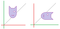
A flip about the line $x=y$ that appeared in the context of finding the graph of the inverse function:

It is given by $$(x,y)\mapsto (y,x).$$

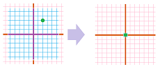
Finally, we have the collapse, a constant function: $$F(x,y)=(x_0,y_0),$$ when the sheet is crushed into a tiny ball:

Of course, any Euclidean space ${\bf R}^n$ can be -- in a similar manner -- rotated (around various axes), stretched (in various directions), projected (onto various lines or planes), or collapsed.

Linear operators

What if we think of these points on the plane as vectors: $$<x,y>\text{ and }<u,v>?$$ Then this is the formula for our function: $$F\big(<x,y> \big) = <u,v> = <2x-3y,x+5y>.$$ Here $<x,y>$ is the input and $<u,v>$ is the output: $$ \newcommand{\ra}[1]{\!\!\!\!\!\xrightarrow{\quad#1\quad}\!\!\!\!\!} \newcommand{\da}[1]{\left\downarrow{\scriptstyle#1}\vphantom{\displaystyle\int_0^1}\right.} % \begin{array}{ccccccccccccccc} \text{input} & & \text{function} & & \text{output} \\ <x,y> & \mapsto & \begin{array}{|c|}\hline\quad f \quad \\ \hline\end{array} & \mapsto & <u,v> \end{array}$$ Both are vectors; it's a vector function!

Warning: We could interpret $F$ as a vector field, but we won't.

Some of the benefits are immediate. For example, the uniform stretch of the plane is simply scalar multiplication: $$F:<x,y>\mapsto k<x,y>.$$

But the real benefit is a better representation of the function: $$F(X) = \left[ \begin{array}{} 2 & -3 \\ 1 & 5 \end{array} \right] \left[ \begin{array}{} x \\ y \end{array} \right] = FX.$$ Turns out, this is the matrix product from first section!

This approach works out but only because $f$ and $g$ happen to be linear.

Exercise. Does it work when the function isn't linear? Try $F(x,y)=(e^x,\frac{1}{y})$.

Conversely, if we do have a matrix, we can always understand it as a function, as follows: $$\left[ \begin{array}{} a & b \\ c & d \end{array} \right] \left[ \begin{array}{} x \\ y \end{array} \right] = \left[ \begin{array}{} ax+by \\ cx+dy \end{array} \right]=<ax+by,cx+dy>,$$ for some $a,b,c,d$ fixed. So matrix $A$ is contains all the information about function $A$. One can think of $A$ (a table) as an abbreviation of $AX$ (a formula).

Warning: We use the same letter for the function and the matrix.

Now, what happens to the vector operations under $A$? Suppose we have addition and scalar multiplication carried out in the domain space of $A$:

Once $A$ has transformed the plane, what do these operations look like now?

At its simplest, an addition diagram rotated will remain an addition diagram:

In other words, addition is preserved under $A$. The same conclusion is quickly reached for the flip and other motions: the triangles of the new diagram are identical to the original. What about the general case?

Consider $A : {\bf R}^2 \to {\bf R}^2$ and two input vectors: $$X=\left[ \begin{array}{} x \\ y \end{array} \right]\text{ and } X'=\left[ \begin{array}{} x' \\ y' \end{array} \right]\ \Longrightarrow\ A(X+X')=?$$ The example suggests the answer: $$A(X+X')=A(X)+A(X').$$ Let's compare: $$\begin{array}{l|l} \text{ LHS: }&\text{ RHS: }\\ A \left( \left[ \begin{array}{} x \\ y \end{array} \right] + \left[ \begin{array}{} x' \\ y' \end{array} \right] \right)&A \left[ \begin{array}{} x \\ y \end{array} \right] + A\left[ \begin{array}{} x' \\ y' \end{array} \right]\\ \begin{array}{} &= \left[ \begin{array}{} a & b \\ c & d \end{array} \right] \left( \left[ \begin{array}{} x \\ y \end{array} \right] + \left[ \begin{array}{} x' \\ y' \end{array} \right] \right) \\ &= \left[ \begin{array}{} a & b \\ c & d \end{array} \right] \left[ \begin{array}{} x + x' \\ y + y' \end{array} \right] \\ &= \left[ \begin{array}{} a(x+x')+b(y+y') \\ c(x+x')+d(y+y') \end{array} \right] \end{array}& \begin{array}{} &= \left[ \begin{array}{} a & b \\ c & d \end{array} \right] \left[ \begin{array}{} x \\ y \end{array} \right] + \left[ \begin{array}{} a & b \\ c & d \end{array} \right] \left[ \begin{array}{} x' \\ y' \end{array} \right] \\ &= \left[ \begin{array}{} ax+by \\ cx+dy \end{array} \right] + \left[ \begin{array}{} ax'+by' \\ cx'+dy' \end{array} \right] \\ &=\left[ \begin{array}{} ax+by+ax'+by' \\ cx + dy + cx' + dy' \end{array} \right] \end{array} \end{array}$$ These are the same, after factoring.

Indeed, the example of a stretch below shows that the triangles of the diagram, if not identical, are similar to the original:

The diagram of scalar multiplication is much simpler. It is a stretch; rotated or stretched, it remains a stretch. To prove, consider an input vector $X=<x,y>$ and a scalar $r$. Then, $$\left[ \begin{array}{} a & b \\ c & d \end{array} \right] \left( r\left[ \begin{array}{} x \\ y \end{array} \right] \right)=\left[ \begin{array}{} a & b \\ c & d \end{array} \right] \left( \left[ \begin{array}{} rx \\ ry \end{array} \right] \right)= \left[ \begin{array}{} arx+bry \\ crx+dry \end{array} \right]= r\left[ \begin{array}{} ax+by \\ cx+dy \end{array} \right]=r\left[ \begin{array}{} a & b \\ c & d \end{array} \right] \left[ \begin{array}{} x \\ y \end{array} \right].$$ In other words, scalar multiplication is preserved under $A$.

Now, this is the general case...

Definition. A function $A:{\bf R}^n\to {\bf R}^m$ that satisfies the following two properties is called a linear operator: $$\begin{array}{ll} A(U+V) &= A(U)+A(V), \\ A(rV) &= rA(V). \end{array}$$

What about dimension $1$? It's $f(x)=ax$.

Warning: Previously, $ax+b$ has been called a “linear function”. Now, $ax$ is called a “linear operator”.

This is the summary.

Theorem. The function $A:{\bf R}^2\to {\bf R}^2$ defined via multiplication by a $2\times 2$ matrix $A$, $$A(X)=AX,$$ is a linear operator. Conversely, every linear operator $A:{\bf R}^2\to {\bf R}^2$ is defined via multiplication by some $2\times 2$ matrix.

Examples of linear operators

We will visualize some examples of linear operators on the plane: $$F:{\bf R}^2\to {\bf R}^2.$$ We illustrate them via compositions. We plot a parametric curve or curves, $X=X(t)$, in the domain and then plot its image in the resulting plane under the transformation $Y=F(X)$. In other words, we plot the image of the function: $$Y=F(X(t)),$$ which is also a parametric curve.

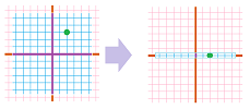
Example (collapse on axis). Let's consider this very simple function: $$\begin{cases}u&=2x\\ v&=0\end{cases} \ \leadsto\ \left[ \begin{array}{} u \\ v \end{array}\right]= \left[\begin{array}{} 2 & 0 \\ 0 & 0 \end{array} \right] \cdot \left[ \begin{array}{} x \\ y \end{array} \right].$$ Below, one can see how this function collapses the whole plane to the $x$-axis:

In the meantime, the $x$-axis is stretched by a factor of $2$. $\square$

Example (stretch-shrink along axes). Let's consider this function: $$\begin{cases}u&=2x\\ v&=4y\end{cases}.$$ Here, this function is given by the matrix: $$F=\left[ \begin{array}{ll}2&0\\0&4\end{array}\right].$$

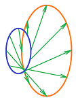
What happens to the rest of the plane? Since the stretching is non-uniform, the vectors turn. However, since the basis vectors $E_1$ and $E_2$ don't turn, this is not a rotation but rather “fanning out” of the vectors:

$\square$

Example (stretch-shrink along axes). A slightly different function is: $$\begin{cases}u&=-x\\ v&=4y\end{cases}. $$ It is simple because the two variables are fully separated.

The slight change to the function produces a similar but different pattern: we see the reversal of the direction of the ellipse around the origin. Here, the matrix of $F$ is diagonal: $$F=\left[ \begin{array}{ll}-1&0\\0&4\end{array}\right].$$ $\square$

Example (collapse). Let's consider a more general function: $$\begin{cases}u&=x&+2y\\ v&=2x&+4y\end{cases} \ \Longrightarrow\ F=\left[ \begin{array}{cc}1&2\\2&4\end{array}\right].$$

It appears that the function is stretching the plane in one direction and collapsing in another. That's why there is a whole line of points $X$ with $FX=0$. To find it, we solve this equation: $$\begin{cases}x&+2y&=0\\ 2x&+4y&=0\end{cases} \ \Longrightarrow\ x=-2y.$$ $\square$

Exercise. Describe what is happening with this matrix $F$: $$F=\left[ \begin{array}{cc}-1&-2\\1&-4\end{array}\right].$$

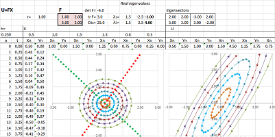
Exercise. Describe what is happening with this matrix $F$: $$F=\left[ \begin{array}{cc}1&2\\3&2\end{array}\right].$$

Example (skewing-shearing). Consider a matrix with repeated (and, therefore, real) eigenvalues: $$F=\left[ \begin{array}{cc}-1&2\\0&-1\end{array}\right].$$ Below, we replace a circle with an ellipse to see what happens to it under such a function:

There is still angular stretch-shrink but this time it is between the two ends of the same line. To see clearer, consider what happens to a square:

The plane is skewed, like a deck of cards:

Another example is when wind blows at the walls with its main force at their top pushing in the direction of the wind while their bottom is held by the foundation. Such a skewing can be carried out with any image editing software such as MS Paint. $\square$

Example (rotation). Consider a rotation through $90$ degrees: $$\begin{cases}u&=& -y\\ v&=x&&\end{cases} \ \leadsto\ \left[\begin{array}{} u \\ v \end{array}\right] = \left[\begin{array}{} 0&1\\-1&0 \end{array}\right] \cdot \left[\begin{array}{} x \\ y \end{array}\right].$$

Consider a rotation through $45$ degrees: $$\begin{cases}u&=\cos \tfrac{\pi}{4} x& -\sin \tfrac{\pi}{4} y\\ v&=\sin \tfrac{\pi}{4} x&+\cos \tfrac{\pi}{4} y& \end{cases} \ \leadsto\ \left[\begin{array}{} u \\ v \end{array}\right] = \left[\begin{array}{rrr} \cos \tfrac{\pi}{4} y & -\sin \tfrac{\pi}{4} y \\ \sin \tfrac{\pi}{4} y & \cos \tfrac{\pi}{4} y \end{array}\right] \cdot \left[\begin{array}{} x \\ y \end{array}\right].$$

$\square$

Example (rotation with stretch-shrink). Let's consider a more complex function: $$\begin{cases}u&=3x&-13y\\ v&=5x&+y\end{cases} .$$ Here, the matrix of $F$ is not diagonal: $$F=\left[ \begin{array}{cc}3&-13\\5&1\end{array}\right].$$

We have a combination of stretching, flipping, and rotating... $\square$

The determinant of a matrix

Let's, once and for all, solve the system of linear equations: $$\begin{cases} ax&+&by&=0,&\quad (1)\\ cx&+&dy&=0.&\quad (2) \end{cases}$$ The system has unspecified coefficients $a,b,c,d$ and the free terms are chosen to be $0$ for simplicity.

From (1), we derive: $$y=-ax/b, \text{ provided }b\ne 0.\quad (3)$$ Substitute this into (2): $$cx+d(-ax/b)=0.$$ Then $$x(c-da/b)=0,$$ or, alternatively, $$x(cb-da)=0, \text{ when }b\ne 0.$$ One possibility is $x=0$; it follows from (3) that $y=0$ too. Then, we have two cases for $b\ne 0$:

• Case 1: $x=0,\ y=0$, or
• Case 2: $ad-bc=0$.

Now, we apply this analysis to $y$ in (1) instead of $x$; we have for $a\ne 0$:

• Case 1: $x=0,\ y=0$, or
• Case 2: $ad-bc=0$.

The result is the same! Furthermore, if we apply this analysis for $x$ and $y$ in (2) instead of (1), we have the same two cases. Thus, whenever one of the four coefficients, $a,b,c,d$, is non-zero, we have these cases:

• Case 1: $x=0,\ y=0$, or
• Case 2: $ad-bc=0$.

But when $a=b=c=d=0$, Case 2 is satisfied... and we can have any values for $x$ and $y$!

Definition. The determinant of a $2\times 2$ matrix is defined to be: $$\det \left[\begin{array}{} a & b \\ c & d \end{array}\right]=ad-bc.$$

What does the determinant determine?

According to the analysis above: $$\det A\ne 0\ \Longrightarrow\ x=y=0.$$ The converse is also true. Indeed, let's consider our system of linear equations again: $$\begin{cases} ax&+&by&=0,&\quad (1)\\ cx&+&dy&=0.&\quad (2) \end{cases}$$ We multiply (1) by $c$ and (2) by $a$. Then we have: $$\begin{cases} cax&+&cby&=0&\quad c(1)\\ acx&+&ady&=0&\quad a(2)\\ \hline (ca-ac)x&+&(cb-ad)y&=0\\ 0\cdot x&-&\det A\cdot y&=0\\ \end{cases}$$ The third equation is the result of subtraction of the first two. The whole equation is zero when $\det A=0$! This means that equations (1) and (2) represent two identical lines. It follows that the original system has infinitely many solutions.

Exercise. What if $a=0$ or $c=0$?

The following is the summary of above analysis.

Theorem. Suppose $A$ is a $2\times 2$ matrix. Then, $\det A\ne 0$ if and only if the solution set of the matrix equation $AX=0$ consists of only $0$.

Thus, the flip, the stretch, and the rotation have non-zero determinants while the projections and the collapse have a zero determinant.

The following is the contra-positive form of the theorem.

Corollary. Suppose $A$ is a $2\times 2$ matrix. Then, there is $X\ne 0$ such that $AX=0$ if and only if $\det A=0$.

Since $A(0)=0$, this indicates that $A$ isn't one-to-one. There is more...

Corollary. A linear operator $A$ is a bijection if and only if $\det A\ne 0$.

Exercise. Prove the rest of the theorem.

So, a zero determinant indicates that some non-zero vector $X$ is taken to $0$ by $A$. It follows that all the multiples, $\lambda X$, of $X$ are also taken to $0$: $$A(\lambda X)=\lambda A(X)=\lambda 0=0.$$ In other words, the whole line is collapsed to $0$. The following may seem less dramatic than that.

Definition. A $2\times 2$ matrix $A$ is called singular when its two columns are multiples of each other.

So, for $$A = \left[\begin{array}{} a & b \\ c & d \end{array}\right],$$ there is such an $x$ that: $$\left[\begin{array}{} a \\ c \end{array}\right] = x\left[\begin{array}{} b \\ d \end{array}\right].$$

Theorem. A $2\times 2$ matrix $A$ is singular if and only if $\det A=0$.

Proof. ($\Rightarrow$) Suppose $A$ is singular, then $$\left[\begin{array}{} a \\ c \end{array}\right] = x \left[\begin{array}{} b \\ d \end{array}\right]\ \Longleftrightarrow\ \begin{cases}a=xb\\ c=xd\end{cases} \Longleftrightarrow\ \det A = ad-bc = (xb)d - b (xd)=0.$$

($\Leftarrow$) Suppose $ad-bc=0$, then let's find $x$, the multiple.

• Case 1: assume $b \neq 0$, then choose $x = \frac{a}{b}$. Then

$$\begin{array}{} xb &= \frac{a}{b}b &= a, \\ xd &= \frac{a}{b}d &= \frac{ad}{b} = \frac{bc}{b} = c. \end{array}$$ So $$x \left[\begin{array}{} b \\ d \end{array}\right] = \left[\begin{array}{} a \\ c \end{array}\right].$$

• Case 2: assume $a \neq 0$... $\blacksquare$

Exercise. Finish the proof.

We make the following observation about determinants, which will reappear in the case of $n\times n$ matrices: the determinant is an alternating sum of terms each of which is the product of $n$ of matrix's entries, exactly one from each row and one from each column.

The following important fact is accepted without proof.

Corollary. The determinant of a linear operator remains the same in any Cartesian coordinate system.

It's a stretch: eigenvalues and eigenvectors

Consider a linear operator given by the matrix: $$A=\left[\begin{array}{} 2 & 0 \\ 0 & 3 \end{array}\right].$$ What exactly does this transformation of the plane do to it? To answer, just consider where $A$ takes the standard basis vectors: $$\begin{array}{} A:& E_1 = \left[\begin{array}{} 1 \\ 0 \end{array}\right] &\mapsto \left[\begin{array}{} 2 \\ 0 \end{array}\right]&=2E_1 \\ A:&E_2 = \left[\begin{array}{} 0 \\ 1 \end{array}\right] &\mapsto \left[\begin{array}{} 0 \\ 3 \end{array}\right]&=3E_2 \end{array}.$$ In other words, what happens to them is scalar multiplication: $$A(E_1)=2E_1\text{ and }A(E_2)=3E_2.$$ So, we can say that $A$ stretches the plane horizontally by a factor of $2$ and vertically by $3$, in either order.

Even though we speak of stretching the plane, this is not to say that vectors are stretched, expect for the vertical and horizontal ones. Indeed, any other vector is rotated; for example, the values of $<1,1>$ isn't its multiple: $$A\left[\begin{array}{} 1 \\ 1 \end{array}\right]=\left[\begin{array}{} 2 \\ 3 \end{array}\right]\ne \lambda \left[\begin{array}{} 1 \\ 1 \end{array}\right],$$ for any real $\lambda$.

In fact, any stretch of this kind will have this form: $$A = \left[\begin{array}{} h & 0 \\ 0 & v \end{array}\right],$$ where $h$ is the horizontal coefficient and $v$ the vertical coefficient.

What about a stretch along other axes? For example, we've seen this:

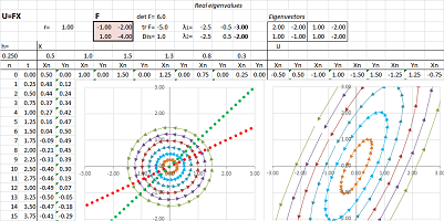
This time the matrix is not diagonal: $$A=\left[ \begin{array}{cc}-1&-2\\1&-4\end{array}\right].$$ The plane is visibly stretched but in what direction or directions? It is hard to tell because the result simply looks skewed.

We know that $A$ rotates some vectors but $A$ acts as scalar multiplication along some -- still unknown -- axes! In other words, if vectors $V_1$ and $V_2$ point along these axes, we have:

• $A(V_1)=\lambda_1 V_1$ and
• $A(V_2)=\lambda_2 V_2$,

for some numbers $\lambda_1$ and $\lambda_2$.

Definition. Given a linear operator $A : {\bf R}^2 \to {\bf R}^2$, a (real) number $\lambda$ is called an eigenvalue of $A$ if $$A(V)=\lambda V,$$ for some non-zero vector $V$ in ${\bf R}^2$. Then, $V$ is called an eigenvector of $A$ corresponding to $\lambda$.

Vector $V=0$ is excluded because we always have $A(0)=0$.

Now, how do we find these?

Example. If this is the identity matrix, $A=I_2$, the equation is easy to solve: $$\lambda V=AV =I_2V=V. $$ So, $\lambda=1$. This is the only eigenvalue. What are its eigenvectors? All vectors but $0$. $\square$

Example. Let's revisit this diagonal matrix: $$A = \left[\begin{array}{ll} 2 & 0 \\ 0 & 3 \end{array}\right].$$ Then our matrix equation becomes: $$\left[\begin{array}{ll} 2 & 0 \\ 0 & 3 \end{array}\right] \left[\begin{array}{ll} x \\ y \end{array}\right] = \lambda \left[\begin{array}{ll} x \\ y \end{array}\right].$$ Let's rewrite: $$\left[\begin{array}{ll} 2x \\ 3y \end{array}\right] = \left[\begin{array}{} \lambda x \\ \lambda y \end{array}\right] \Longrightarrow\ \begin{cases} 2x &=\lambda x \\ 3y &= \lambda y\\ \end{cases} \Longrightarrow\ \begin{cases} x(2-\lambda ) &=0,&\quad (1) \\ y(3-\lambda ) &=0.&\quad (2) \\ \end{cases}$$ Now, we have $V=<x,y>\ne 0$, so either $x\ne 0$ or $y\ne 0$. Let's use the above equations to consider these two cases:

• Case 1: $x \ne 0$, then from (1), we have: $2-\lambda =0 \Longrightarrow \lambda =2$,
• Case 2: $y \ne 0$, then from (2), we have: $3-\lambda =0 \Longrightarrow \lambda =3$.

These are the only two possibilities. So, if $\lambda = 2$, then $y=0$ from (2). Therefore, the corresponding eigenvectors are: $$\left[\begin{array}{} x \\ 0 \end{array}\right],\ x \neq 0.$$ If $\lambda=3$, then $x=0$ from (1). Therefore, the corresponding eigenvectors are: $$\left[\begin{array}{ll} 0 \\ y \end{array}\right],\ y \neq 0.$$ These two sets are almost equal to the two axes! If we append $0$ to these sets of eigenvectors, we have the following. For $\lambda = 2$, the set is the $x$-axis: $$\left\{ \left[\begin{array}{ll} x \\ 0 \end{array}\right] :\ x \text{ real } \right\}.$$ And for $\lambda=3$, the set is the $y$-axis: $$\left\{\left[\begin{array}{ll} 0 \\ y \end{array}\right] :\ y \text{ real } \right\}.$$ $\square$

Definition. For a (real) eigenvalue $\lambda$ of $A$, the eigenspace of $A$ corresponding to $\lambda$ is defined and denoted by the following: $$E(\lambda) = \{ V :\ A(V)=\lambda V \}.$$

It's all eigenvectors of $\lambda$ plus $0$...

Example. For the identity matrix, we have: $$E_{I_2}(1) = {\bf R}^2.$$ $\square$

Example. For $$A = \left[ \begin{array}{} 2 & 0 \\ 0 & 3 \end{array}\right],$$ we have:

• $E(2)$ is $x$-axis.
• $E(3)$ is $y$-axis.

$\square$

Example. For the zero matrix, $A=0$, we have $$AV=\lambda V, \text{ or } 0 = \lambda V.$$ Therefore, $\lambda =0$. Hence $$E(0)={\bf R}^2.$$ $\square$

Example. Consider now the projection on the $x$-axis, $$P = \left[\begin{array}{} 1 & 0 \\ 0 & 0 \end{array}\right].$$ Then our matrix equation is solved as follows: $$\left[\begin{array}{} 1 & 0 \\ 0 & 0 \end{array} \right] \left[ \begin{array}{} x \\ y \end{array} \right] = \lambda \left[\begin{array}{} x \\ y \end{array}\right] \Longrightarrow\ \left[\begin{array}{} x \\ 0 \end{array}\right] = \left[\begin{array}{} \lambda x \\ \lambda y \end{array}\right] \Longrightarrow\ \begin{cases} x=\lambda x\\ 0 =\lambda y\end{cases}.$$ So, the only possible cases are: $$\lambda =0 \text{ and } \lambda=1.$$

Next, in order to find the corresponding eigenvalues, we now go back to the system of linear equations for $x$ and $y$. We consider these two cases. Case 1:

• $\lambda = 0 \Longrightarrow $
• $x=0 \cdot x \Longrightarrow x=0$, and
• $0=0 \cdot y \Longrightarrow y$ any.

Hence, $$E(0) = \left\{ \left[\begin{array}{lll} 0 \\ y \end{array}\right] :\ y \text{ real} \right\}.$$ This is the $y$-axis. Case 2:

• $\lambda = 1 \Longrightarrow $
• $x=1 \cdot x \Longrightarrow x$ any, and
• $0=1 \cdot y \Longrightarrow y=0$.

Hence, $$E(1) = \left\{ \left[\begin{array}{lll} x \\ 0 \end{array}\right] :\ x \text{ real} \right\}.$$ This is the $x$-axis. $\square$

Example. Suppose $A$ is the $90$ degree rotation: $$A = \left[\begin{array}{} 0 & -1 \\ 1 & 0 \end{array}\right].$$ Then, to find the eigenvalues, we solve this system of linear equations: $$\left[\begin{array}{} 0 & -1 \\ 1 & 0 \end{array}\right] \left[\begin{array}{} x \\ y \end{array}\right] = \lambda \left[\begin{array}{} x \\ y \end{array} \right]\ \Longrightarrow\ \begin{cases} -y &= \lambda x \\ x &= \lambda y \end{cases} \Longrightarrow\ \begin{cases} -xy &= \lambda x^2 \\ xy &= \lambda y^2 \end{cases} \ \Longrightarrow\ \lambda x^2 = -\lambda y^2\ \Longrightarrow\ x^2=-y^2 \text{ or }\lambda=0.$$ A direct examination reveals that $\lambda = 0$ is not an eigenvalue. In the meantime, the equation $x^2=-y^2$ is impossible! There seems to be no eigenvalues, certainly not real ones... $\square$

Example. Let's revisit this linear operator: $$A=\left[ \begin{array}{cc}-1&-2\\1&-4\end{array}\right].$$ Our equation becomes: $$\left[\begin{array}{} -1 & -2 \\ 1 & -4 \end{array}\right] \left[\begin{array}{} x \\ y \end{array}\right] = \lambda \left[\begin{array}{} x \\ y \end{array}\right].$$ Let's rewrite: $$\left[\begin{array}{} -x-2y \\ x-4y \end{array}\right] = \left[\begin{array}{} \lambda x \\ \lambda y \end{array}\right] \Longrightarrow \begin{cases} (-1-\lambda)x&-&2y &=0 \\ x&+&(-4-\lambda )y &= 0\\ \end{cases}.$$ This is another system of linear equations to be solved, again. Is there an easier way? $\square$

Let's try an alternative approach...

Suppose $\lambda$ is an eigenvalue for matrix $A$. This means that, for some non-zero vector $V$ in ${\bf R}^2$, we try to rewrite our matrix equation: $$AV=\lambda V\ \Longleftrightarrow\ AV-\lambda V = 0 \ \Longleftrightarrow\ (A-\lambda)V=0 ?$$ But $\lambda$ is a number not a matrix! The last equation is better rewritten as: $$ AV-\lambda V=0\ \Longleftrightarrow\ AV-\lambda I_2V=0\ \Longleftrightarrow\ (A-\lambda I_2)V=0.$$ This is a new matrix equation to be solved:

• the matrix is $F=A - \lambda I_2$,
• $V$ is the unknown,
• the right hand side is $B=0$.

But do we really need to solve it? Our strategy is to go after the eigenvalues initially and the to find the eigenvectors. Then, all we need is the following familiar theorem: there is a non-zero solution of $FX=0$ if and only if the determinant of the matrix is zero, $\det F = 0$.

Theorem. Suppose $A$ is a linear operator ${\bf R}^2$. Then an eigenvalue $\lambda$ of $A$ is a solution to the following (quadratic) equation: $$\det (A-\lambda I_2)=0.$$

Note: “Eigen” means “characteristic” in German.

Definition. The characteristic polynomial of an $2\times 2$ matrix $A$ is defined to be: $$\chi_A(\lambda) = \det(A - \lambda I_2).$$

Meanwhile, the equation is called the characteristic equation.

Example. Consider again: $$A = \left[\begin{array}{} 2 & 0 \\ 0 & 3 \end{array}\right],$$ then $$\chi_A(\lambda) = \det \left[\begin{array}{} 2-\lambda & 0 \\ 0 & 3-\lambda \end{array}\right] = (2-\lambda)(3-\lambda) = 0.$$ Therefore, we have: $$\lambda=2,\ 3.$$ $\square$

Example. If $$A=\left[\begin{array}{} 1 & 0 \\ 0 & 0 \end{array}\right],$$ the characteristic equation is: $$\chi_A(\lambda) = \det \left[\begin{array}{} 1-\lambda & 0 \\ 0 & \lambda \end{array}\right] = (1-\lambda)\lambda = 0.$$ Then, $$\lambda=1,\ 0.$$ $\square$

Example. Take $A$ the $90$ degree rotation again. Then, $$\chi_A(\lambda) = \det \left[\begin{array}{} -\lambda & -1 \\ 1 & -\lambda \end{array}\right] = \lambda^2+1 = 0.$$ No real solutions! So, no vector is taken by $A$ to its own multiple. $\square$

A broader view is provided by the theorem below.

Theorem. If $A$ is an $2 \times 2$ matrix, then

• the eigenvalues are the real roots of the (quadratic) characteristic polynomial $\chi_A$, and, therefore,
• the number of eigenvalues is less than or equal to $2$, counting their multiplicities.

Linear operators with real eigenvalues

We have shown how one can understand the way a linear operator transforms the plane: by examining what happens to the various curves. This time, we would like to learn how to predict the outcome by examining only its matrix.

Below is a familiar fact that will take us down that road.

Theorem. When $\det F\ne 0$, the vector $X=0$ is the only vector that give the zero value under the operator $Y=FX$; otherwise, there are infinitely many such points.

In other words, what matters is whether $F$, as a function, is or is not one-to-one.

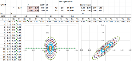
Example (collapse on axis). The latter is the “degenerate” case such as the following: $$\begin{cases}u&=2x\\ v&=0\end{cases} \ \leadsto\ \left[ \begin{array}{} u \\ v \end{array}\right]= \left[\begin{array}{} 2 & 0 \\ 0 & 0 \end{array} \right] \, \left[ \begin{array}{} x \\ y \end{array} \right].$$ Below, one can see how this function collapses the whole plane to the $x$-axis while the $x$-axis is stretched by a factor of $2$:

$\square$

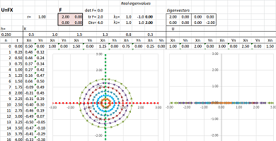
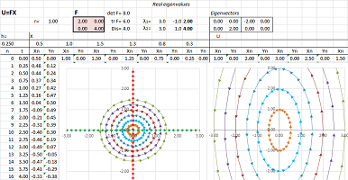
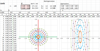
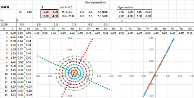
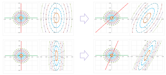
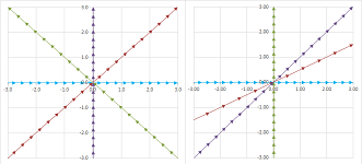
The illustrations are produced by a spreadsheet. By mapping various curves, one can see how the linear operator given by this matrix transforms the plane: stretching, shrinking in various directions, rotations, etc. The spreadsheet also shows eigenspaces as two (or one, or none) straight lines; they remain in place under the transformation. Running a few examples demonstrates a classification of matrices, which in turn will give us -- in Chapter 24 -- a classification of systems of ODEs...

Example (stretch-shrink along axes). Let's consider this linear operator and its matrix $$\begin{cases}u&=2x\\ v&=4y\end{cases} \text{ and } F=\left[ \begin{array}{ll}2&0\\0&4\end{array}\right].$$ To see the transformation of the whole plane, we see first the transformations of the two axes. In other words, we track the values of the basis vectors and the rest of the values are seen as a linear combination of these.

The vectors turn non-uniformly, i.e., they “fan out”:

Algebraically, we have: $$FX=F\left[ \begin{array}{ll}u\\v\end{array}\right]=u \left[ \begin{array}{ll}2\\0\end{array}\right] +v\left[ \begin{array}{ll}0\\4\end{array}\right]=2u \left[ \begin{array}{ll}1\\0\end{array}\right] +4v\left[ \begin{array}{ll}0\\1\end{array}\right]=uE_1+4vE_2.$$ The last expression is a linear combination of the values of the two standard basis vectors. The middle, however, is also a linear combination but with respect to two “non-standard” basis vectors: $$V_1=\left[ \begin{array}{ll}2\\0\end{array}\right] \text{ and } V_2=\left[ \begin{array}{ll}0\\4\end{array}\right].$$ $\square$

Example (stretch-shrink along axes). A slightly different function is: $$\begin{cases}u&=-x\\ v&=4y\end{cases} \text{ and } F=\left[ \begin{array}{ll}-1&0\\0&4\end{array}\right]. $$ It is still simple because the two variables remain fully separated. We can think of either of these two transformations as a transformation of the whole plane that is limited to one of the two axes:

The slight change to the function produces a similar but different pattern: we see the reversal of the direction of the ellipse around the origin. Algebraically, we have as before: $$FX=F\left[ \begin{array}{ll}u\\v\end{array}\right]= u\left[ \begin{array}{ll}-1\\0\end{array}\right] +v\left[ \begin{array}{ll}0\\4\end{array}\right]=- u\left[ \begin{array}{ll}1\\0\end{array}\right] +4v\left[ \begin{array}{ll}0\\1\end{array}\right]=-uE_1+4vE_2.$$ Once again, the last expression is a linear combination of the values of the two standard basis vectors while the middle is a linear combination but with respect to another basis: $$V_1=\left[ \begin{array}{ll}-1\\0\end{array}\right] \text{ and } V_2=\left[ \begin{array}{ll}0\\4\end{array}\right].$$ $\square$

What if the two variables aren't separated? In the examples, the standard basis vectors happen to be the eigenvectors of the two (diagonal) matrices. The insight provided by the examples is that the two variables can be separated -- along the eigenvectors of the matrix that serve as an alternative basis. To see how this happens, just imagine that the two pictures above are skewed (the latter also reverses the orientation of the curve):

The idea is uncomplicated: the linear operator within the eigenspace is $1$-dimensional. It can then be represented the usual way -- by a single number. If we know this number, how do we find the rest of the values of the linear operator? In two steps. First, every $X$ that lies within the eigenspace, which is a line, is a multiple of the eigenvector and its value under $F$ can be easily computed: $$X=rV\ \Longrightarrow\ U=F(rV)=rFV=r\lambda V.$$ In fact, we have the following result.

Theorem (Eigenspaces). If $\lambda$ is a (real) eigenvalue and $V$ a corresponding eigenvector of a matrix $F$, then every multiple of $V$ is also an eigenvector; i.e., $$V \text{ belongs to } E(\lambda) \ \Longrightarrow\ U=r V \text{ belongs to } E(\lambda) \text{ for any real } r.$$

Second, the rest of values is covered by the following idea: try to express the value as a linear combination of two values found so far. In fact, we have the following result.

Theorem (Representation). Suppose $V_1$ and $V_2$ are two eigenvectors of a matrix $F$ that correspond to two (possibly equal) eigenvalues $\lambda_1$ and $\lambda_2$. Suppose also that $V_1$ and $V_2$ aren't multiples of each other. Then, all values of the linear operator $Y=FX$ are represented as linear combinations of its values on the eigenvectors: $$X=cV_1+kV_2\ \Longrightarrow\ FX=c\lambda_1V_1+k\lambda_2V_2,$$ with some real coefficients $C$ and $K$.

Exercise. Show that when all eigenvectors are multiples of each other, the formula won't give us all the values of the linear operator.

Let's consider a few functions with non-diagonal matrices.

Example (collapse). Let's consider a more general linear operator: $$\begin{cases}u&=x&+&2y\\ v&=2x&+&4y\end{cases} \ \Longrightarrow\ F=\left[ \begin{array}{cc}1&2\\2&4\end{array}\right].$$

It appears that the function has a stretching in one direction and a collapse in another. What are those directions? Linear algebra gives the answer.

First, the determinant is zero: $$\det F=\det\left[ \begin{array}{cc}1&2\\2&4\end{array}\right]=1\cdot 4-2\cdot 2=0.$$ That's why there is a whole line of points $X$ with $FX=0$. To find it, we solve this equation: $$\begin{cases}x&+&2y&=0\\ 2x&+&4y&=0\end{cases} \ \Longrightarrow\ x=-2y.$$ We have, then, eigenvectors corresponding to the zero eigenvalue $\lambda_1=0$: $$V_1=\left[\begin{array}{cc}2\\-1\end{array}\right]\ \Longrightarrow\ FV_1=0 .$$

So, second, there is only one non-zero eigenvalue: $$\det (F-\lambda I)=\det\left[ \begin{array}{cc}1-\lambda&2\\2&4-\lambda\end{array}\right]=\lambda^2-5\lambda=\lambda(\lambda-5).$$ Let's find the eigenvectors for $\lambda_2=5$. We solve the equation: $$FV=\lambda_2 V,$$ as follows: $$FV=\left[ \begin{array}{cc}1&2\\2&4\end{array}\right]\left[\begin{array}{cc}x\\y\end{array}\right]=5\left[\begin{array}{cc}x\\y\end{array}\right].$$ This gives as the following system of linear equations: $$\begin{cases}x&+&2y&=5x\\ 2x&+&4y&=5y\end{cases} \ \Longrightarrow\ \begin{cases}-4x&+&2y&=0\\ 2x&-&y&=0\end{cases} \ \Longrightarrow\ y=2x.$$ This line is the eigenspace. We choose the eigenvector to be: $$V_2=\left[\begin{array}{cc}1\\2\end{array}\right].$$

Every value is a linear combination of the values of the two eigenvectors: $$X=c\, V_1+k\, V_2 \ \Longrightarrow\ FX=c\left[\begin{array}{cc}2\\-1\end{array}\right]+k\cdot 0\cdot\left[\begin{array}{cc}1\\2\end{array}\right].$$ $\square$

Exercise. Find the line of the projection.

Example (stretch-shrink). Let's consider this function: $$\begin{cases}u&=-x&-&2y,\\ v&=x&-&4y.\end{cases} $$ Here, the matrix of $F$ is not diagonal: $$F=\left[ \begin{array}{cc}-1&-2\\1&-4\end{array}\right].$$

The analysis starts with the characteristic polynomial: $$\det (F-\lambda I)=\det \left[ \begin{array}{cc}-1-\lambda&-2\\1&-4-\lambda\end{array}\right]=\lambda^2-5\lambda+6.$$ Therefore, the eigenvalues are: $$\lambda_1=-3,\ \lambda_2=-2.$$

To find the eigenvectors, we solve the two equations: $$FV_i=\lambda_i V_i,\ i=1,2.$$ The first: $$FV_1=\left[ \begin{array}{cc}-1&-2\\1&-4\end{array}\right]\left[\begin{array}{cc}x\\y\end{array}\right]=-1\left[\begin{array}{cc}x\\y\end{array}\right].$$ This gives as the following system of linear equations: $$\begin{cases}-x&-&2y&=-3x\\ x&-&4y&=-3y\end{cases} \ \Longrightarrow\ \begin{cases}2x&-&2y&=0\\ x&-&y&=0\end{cases} \ \Longrightarrow\ x=y.$$ We choose: $$V_1=\left[\begin{array}{cc}1\\1\end{array}\right].$$

The second eigenvalue: $$FV_2=\left[ \begin{array}{cc}-1&-2\\1&-4\end{array}\right]\left[\begin{array}{cc}x\\y\end{array}\right]=-2\left[\begin{array}{cc}x\\y\end{array}\right].$$ We have the following system: $$\begin{cases}-x&-&2y&=-2x\\ x&-&4y&=-2y\end{cases} \ \Longrightarrow\ \begin{cases}x&-&2y&=0\\ x&-&2y&=0\end{cases}\ \Longrightarrow\ x=2y.$$ We choose: $$V_2=\left[\begin{array}{cc}2\\1\end{array}\right].$$

Then, $$X=c\, V_1+k\, V_2 \ \Longrightarrow\ FX=-3c\, \left[\begin{array}{cc}2\\-1\end{array}\right]-2k\,\left[\begin{array}{cc}1\\2\end{array}\right].$$ $\square$

Example (stretch-shrink). Let's consider this linear operator: $$\begin{cases}u&=x&+&2y,\\ v&=3x&+&2y.\end{cases} $$ Here, the matrix of $F$ is not diagonal: $$F=\left[ \begin{array}{cc}1&2\\3&2\end{array}\right].$$

Let's find the eigenvectors: $$\det (F-\lambda I)=\det \left[ \begin{array}{cc}1-\lambda&2\\3&2-\lambda\end{array}\right]=\lambda^2-3\lambda-4.$$ Therefore, the eigenvalues are: $$\lambda_1=-1,\ \lambda_2=4.$$

Now we find the eigenvectors. We solve the two equations: $$FV_i=\lambda_i V_i,\ i=1,2.$$ The first: $$FV_1=\left[ \begin{array}{cc}1&2\\3&2\end{array}\right]\left[\begin{array}{cc}x\\y\end{array}\right]=-1\left[\begin{array}{cc}x\\y\end{array}\right].$$ This gives as the following system of linear equations: $$\begin{cases}x&+&2y&=-x\\ 3x&+&2y&=-y\end{cases} \ \Longrightarrow\ \begin{cases}2x&+&2y&=0\\ 3x&+&3y&=0\end{cases} \ \Longrightarrow\ x=-y.$$ We choose: $$V_1=\left[\begin{array}{cc}1\\-1\end{array}\right].$$ Every value within this eigenspace (the line $y=-x$) is a multiple of this eigenvector: $$X=\lambda_1V_1=-\left[\begin{array}{cc}1\\-1\end{array}\right].$$

The second eigenvalue: $$FV_2=\left[ \begin{array}{cc}1&2\\3&2\end{array}\right]\left[\begin{array}{cc}x\\y\end{array}\right]=4\left[\begin{array}{cc}x\\y\end{array}\right].$$ We have the following system: $$\begin{cases}x&+&2y&=4x\\ 3x&+&2y&=4y\end{cases} \ \Longrightarrow\ \begin{cases}-3x&+&2y&=0\\ 3x&-&2y&=0\end{cases}\ \Longrightarrow\ x=2y/3.$$ We choose: $$V_2=\left[\begin{array}{cc}1\\3/2\end{array}\right].$$ Every value within this eigenspace (the line $y=3x/2$) is a multiple of this eigenvector: $$X=\lambda_2V_2=4\left[\begin{array}{cc}1\\3/2\end{array}\right].$$

Then, $$X=c\, V_1+k\, V_2 \ \Longrightarrow\ U=FX=-c\left[\begin{array}{cc}1\\-1\end{array}\right]+4k\left[\begin{array}{cc}1\\3/2\end{array}\right].$$ $\square$

Let's summarize the results.

Theorem (Classification of linear operators -- real eigenvalues). Suppose matrix $F$ has two real non-zero eigenvalues $\lambda _1$ and $\lambda_2$. Then, the function $U=FX$ stretches/shrinks each eigenspace by a factor $|\lambda _1|$ and $|\lambda_2|$ respectively and

• if $\lambda _1$ and $\lambda_2$ have the same sign, it preserves the orientation of a closed curve around the origin; and
• if $\lambda _1$ and $\lambda_2$ have the opposite signs, it reverses the orientation of a closed curve around the origin.

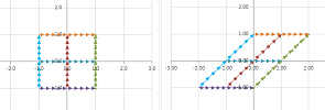
Example (skewing-shearing). Consider a matrix with repeated (and, therefore, real) eigenvalues: $$F=\left[ \begin{array}{cc}1&1\\0&1\end{array}\right].$$ Below, we replace a circle with an ellipse to see what happens to it under such a function:

There is still angular stretch-shrink but this time it is between the two ends of the same line. We see “fanning out” again:

To see clearer, consider what happens to a square:

This is the characteristic polynomial: $$\det (F-\lambda I)=\det \left[ \begin{array}{cc}1-\lambda&1\\0&1-\lambda\end{array}\right]=(1-\lambda)^2.$$ Therefore, the eigenvalues are $$\lambda_1=\lambda_2=1.$$ What are the eigenvectors? $$FV_{1,2}=\left[ \begin{array}{cc}1&1\\0&1\end{array}\right]\left[\begin{array}{cc}x\\y\end{array}\right]=1\left[\begin{array}{cc}x\\y\end{array}\right].$$ This gives as the following system of linear equations: $$\begin{cases}x&+&y&=x\\ &&y&=y\end{cases} \ \Longrightarrow\ x \text{ any},\ y=0.$$ The only eigenvectors are horizontal! Therefore, our classification theorem doesn't apply... $\square$

Example. There are even more outcomes that the theorem doesn't cover. Recall the characteristic polynomial of the matrix $A$ of the $90$ degree rotation: $$\chi_A(\lambda) = \det \left[\begin{array}{} -\lambda & -1 \\ 1 & -\lambda \end{array}\right] = \lambda^2+1.$$ But the characteristic equation, $$x^2+1=0,$$ has no real solutions! Are we done then?.. $\square$

How complex numbers emerge

The equation $$x^2+1=0$$ has no solutions. Indeed, if we try to solve it the usual way, we get these: $$x=\sqrt{-1} \text{ and } x=-\sqrt{-1}.$$ There are no such real numbers! However, let's ignore this fact for a moment. Let's substitute what we have back into the equation and -- blindly -- follow the rules of algebra. We “confirm” that this “number” is a “solution”: $$x^2+1=(\sqrt{-1})^2+1=(-1)+1=0.$$

We call this entity the imaginary unit, denoted by $i$.

We just add this “number” to the set of numbers we do algebra with:

And see what happens...

The only thing we need to know about $i$ is this four-part convention:

• $i$ is not a real number, but
• $i$ can participate in the (four) algebraic operations with real numbers by following the same rules;
• $i^2=-1$ and, consequently,
• $i\ne 0$.

We use these fundamental facts and replace $\sqrt{-1}$ with $i$ any time we want.

Using these rules, we discover that our irreducible (Chapter 4) polynomial can now be factored: $$(x-i)(x+i)=x^2-ix+ix-i^2=x^2+1.$$

Warning: $i$ is not an $x$-intercept of $f(x)=x^2+1$ as the $x$-axis (“the real line”) consists of only (and all) real numbers.

Definition. The multiples of the imaginary unit, $2i,-i,...$, are called imaginary numbers.

We have created a whole class of non-real numbers! There are as many of them as the real numbers:

Except $0i=0$ is real!

Example. The imaginary numbers may also come from solving the simplest quadratic equations. For example, the equation $$x^2+4=0$$ gives us via our substitution: $$x=\pm\sqrt{-4}=\pm \sqrt{4}\sqrt{-1}=\pm 2i.$$ Indeed, if we substitute $2i$ into $$x^2+4=0,$$ we have: $$(2i)^2+4=-4+4=0.$$ $\square$

Imaginary numbers obey the laws of algebra as we know them! If we need to simplify the expression, we try to manipulate it in such a way that real numbers are combines with real while $i$ is pushed aside.

For example, we can just factor $i$ out of all addition and subtraction: $$5i+3i=(5+3)i=8i.$$ It looks exactly like middle school algebra: $$5x+3x=(5+3)x=8x.$$ After all, $x$ could be $i$. The nature of the unit doesn't matter (if we can push it aside): $$5\text{ in.}+3\text{ in.}=(5+3)\text{ in.}=8\text{ in.},$$ or $$5\text{ apples }+3\text{ apples }=(5+3)\text{ apples }=8\text{ apples }.$$ It's “$8$ apples” not “$8$”! And so on.

This is how we multiply an imaginary number by a real number: $$2\cdot(3i)=(2\cdot 3)i=6i.$$

How do we multiply two imaginary numbers? In contrast to the above, even though multiplication and division follow the same rule as always, we can, when necessary, and often have to, simplify the outcome of our algebra using our fundamental identity: $$i^2=-1.$$ For example: $$(5i)\cdot(3i)=(5\cdot 3) (i\cdot i)=15i^2=15(-1)=-15.$$

We also simplify the outcome using the other fundamental fact about the imaginary unit: $$i\ne 0.$$ We can divide by $i$! For example, $$\frac{5i}{3i}=\frac{5}{3}\frac{i}{i}=\frac{5}{3}\cdot 1=\frac{5}{3}.$$

As you can see, doing algebra with imaginary numbers will often bring us back to real numbers. These two classes of numbers cannot be separated from each other!

They aren't. Let's take another look at quadratic equations. The equation $$ax^2+bx+c=0, \ a\ne 0,$$ is solved with the familiar Quadratic Formula: $$x=\frac{-b\pm\sqrt{b^2-4ac}}{2a}.$$ Let's consider $$x^2+2x+10=0.$$ Then the roots are supposed to be: $$\begin{array}{ll} x&=\frac{-2\pm\sqrt{2^2-4\times 10}}{2}\\ &=\frac{-2\pm\sqrt{-36}}{2}\\ &=-1\pm\sqrt{-9}\\ &=-1\pm\sqrt{9}\sqrt{-1}\\ &=-1\pm 3i. \end{array}$$ We end up adding real and imaginary numbers!

Warning: there is no way to simplify this.

This addition is not literal. It's like “adding” apples to oranges: $$5\text{ apples }+3\text{ oranges }=...$$ It's not $8$ and it's not $8$ fruit because we wouldn't be able to read this equality backwards. The algebra is still possible: $$(5a+3o)+(2a+4o)=(5+3)a+(3+4)o=8a+7o.$$ Or, something familiar: $$(5+3x)+(2+4x)=(5+3)+(3+4)=8a+7x,$$ and something new: $$(5+3i)+(2+4i)=(5+3)+(3+4)i=8+7i.$$

The number we are facing consist of both real numbers and imaginary numbers. This fact makes them “complex”...

Definition. Any sum of real and imaginary numbers is called a complex number. The set of all complex numbers is denoted by ${\bf C}$.

Warning: all real numbers are complex!

Addition and subtraction are easy; we just combine similar terms just like in middle school. For example, $$(1+5i)+(3-i)=1+5i+3-i=(1+4)+(5i-i)=5+4i.$$

To simplify multiplication of complex numbers, we expand and then use $i^2=-1$, as follows: $$\begin{array}{ll} (1+5i)\cdot (3-i)&=1\cdot 3+5i\cdot 3+1\cdot(-i)+5i\cdot (-i)\\ &=3+15i-i-5i^2\\ &=(3+5)+(15i-i)\\ &=8+14i. \end{array}$$

It's a bit trickier with division: $$\begin{array}{ll} \frac{1+5i}{3-i}&=\frac{1+5i}{3-i}\frac{3+i}{3+i}\\ &=\frac{(1+5i)(3+i)}{(3-i)(3+i)}\\ &=\frac{-2+8i}{3^2-i^2}\\ &=\frac{-2+8i}{3^2+1}\\ &=\frac{1}{10}(-2+8i)\\ &=-.2+.8i.\\ \end{array}$$ The simplification of the denominator is made possible by the trick of multiplying by $3+i$. It is the same trick we used in Chapters 5 and 6 to simplify fractions with roots to compute their limits: $$\frac{1}{1-\sqrt{x}}=\frac{1}{1-\sqrt{x}}\frac{1+\sqrt{x}}{1+\sqrt{x}}=\frac{1+\sqrt{x}}{1-x}.$$

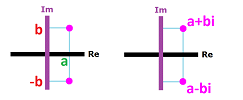
Definition. The complex conjugate of $z=a+bi$ is defined and denoted by: $$\bar{z}=\overline{a+bi}=a-bi.$$

The following is crucial.

Theorem (Algebra of complex numbers). The rules of the algebra of complex numbers are identical to those of real numbers:

• Commutativity of addition: $z+u=u+z$;
• Associativity of addition: $(z+u)+v=z+(u+v)$;
• Commutativity of multiplication: $z\cdot u=u\cdot z$;
• Associativity of multiplication: $(z\cdot u)\cdot v=z\cdot (u\cdot v)$;
• Distributivity: $z\cdot (u+ v)=z\cdot u+ z \cdot v$.

This is the complex number system; it follows the rules of the real number system but also contains it. This theorem will allow us to build calculus for complex functions that is almost identical to that for real functions and also contains it.

Definition. Every complex number $x$ has the standard representation: $$z=a+bi,$$ where $a$ and $b$ are two real numbers. The two components are named as follows:

• $a$ is the real part of $z$, with notation $a=\operatorname{Re}(z)$, and
• $bi$ is the imaginary part of $z$, with notation $b=\operatorname{Im}(z)$.

Then, the purpose of the computations above were to find the standard form of a complex number that comes from algebraic operations with other complex numbers.

So, complex numbers are linear combinations of the real unit, $1$, and the imaginary unit, $i$. This representation helps us understand that two complex numbers are equal if and only if both their real and imaginary parts are equal. Thus, $$z=\operatorname{Re}(z)+\operatorname{Im}(z)i.$$

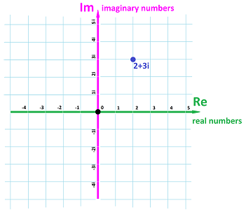
In order to see the geometric representation of complex numbers we need to combine the real number line and the imaginary number line. How? We realize that that have nothing in common... except $0=0i$ belongs to both! We then unite them in the same manner we built the $xy$-plane in Chapter 2:

It is called the the complex plane, ${\bf C}$.

If $z=a+bi$, then $a$ and $b$ are thought of as the components of vector $z$ in the plane. We have a one-to-one correspondence: $${\bf C}\longleftrightarrow {\bf R}^2,$$ given by $$a+bi\longleftrightarrow <a,b>.$$

Then the $x$-axis of this plane consists of the real numbers and the $y$-axis of the imaginary numbers.

Then the complex conjugate of $z$ is the complex number with the same real part as $z$ and the imaginary part with the opposite sign: $$\operatorname{Re}(\bar{z})=\operatorname{Re}(z) \text{ and } \operatorname{Im}(\bar{z})=-\operatorname{Im}(z).$$

Warning: all numbers we have encountered in this book so far are real non-complex, and so are all quantities one can encounter in day-to-day life or science: time, location, length, area, volume, mass, temperature, money, etc.

Classification of quadratic polynomials

The general quadratic equation with real coefficients, $$ax^2+bx+c=0, \ a\ne 0,$$ can be simplified. Let's divide by $a$ and study the resulting quadratic polynomial: $$f(x)=x^2+px+q,$$ where $p=b/a$ and $q=c/a$. The Quadratic Formula then provides the $x$-intercepts of this function: $$x=-\frac{p}{2}\pm\frac{\sqrt{p^2-4q}}{2}.$$ Of course, the $x$-intercepts are the real solutions of this equation and that is why the result only makes sense when the discriminant of the quadratic polynomial, $$D=p^2-4q,$$ is non-negative.

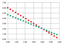
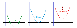
Now, increasing the value of $q$ makes the graph of $y=f(x)$ shift upward and, eventually, pass the $x$-axis entirely. We can observe how its two $x$-intercepts start to get closer to each other, then merge, and finally disappear:

This process is explained by what is happening, with the growth of $q$, to the roots given by the Quadratic Formula: $$x_{1,2}=-\frac{p}{2}\pm\frac{\sqrt{D}}{2}.$$

• Starting with a positive value, $D$ decreases and $\frac{\sqrt{D}}{2}$ decreases; then
• $D=0$ and $\frac{\sqrt{D}}{2}=0$; then
• $D$ becomes negative and $\frac{\sqrt{D}}{2}$ becomes imaginary (but $\frac{\sqrt{-D}}{2}$ is real).

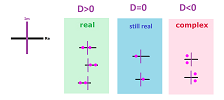
The roots are, respectively: $$\begin{array}{l|ll} \text{discriminant }&\text{ root }\# 1&\quad&\text{ root }\# 2\\ \hline D>0&x_{1}=-\frac{p}{2}-\frac{\sqrt{D}}{2} && x_2=-\frac{p}{2}+\frac{\sqrt{D}}{2}\\ D=0&x_{1}=-\frac{p}{2} && x_2=-\frac{p}{2}\\ D<0&x_{1}=-\frac{p}{2}-\frac{\sqrt{-D}}{2}i && x_2=-\frac{p}{2}+\frac{\sqrt{-D}}{2}i \end{array}$$ Observe that the real roots ($D>0$) are unrelated while the complex ones ($D<0$) are linked so much that knowing one tells us what the one is: just flip the sign; they are conjugate of each other:

They always come in pairs!

As a summary, we have the following classification the roots of quadratic polynomials in terms of the sign of the discriminant.

Theorem (Classification of Roots I). The two roots of a quadratic polynomial with real coefficients are:

• distinct real when its discriminant $D$ is positive;
• equal real when its discriminant $D$ is zero;
• complex conjugate of each other when its discriminant $D$ is negative.

To understand ODEs, we will need a more precise way to classify the polynomials: according to the signs of the real parts of their roots. The signs will determine increasing and decreasing behavior of certain solutions. Once again, these are the possibilities:

Theorem (Classification of Roots II). Suppose $x_1$ and $x_2$ are the two roots of a quadratic polynomial $f(x)=x^2+px+q$ with real coefficients. Then the signs of the real parts $\operatorname{Re}(x_1)$ and $\operatorname{Re}(x_2)$ of $x_1$ and $x_2$ are:

• same when $p^2> 4q$ and $q\ge 0$;
• opposite when $p^2> 4q$ and $q<0$;
• same and opposite of that of $p$ when $p^2\le 4q$.

Proof. The condition $p^2\le 4q$ is equivalent to $D\le 0$. We can see in the table above that, in that case, we have $\operatorname{Re}(x_1)=\operatorname{Re}(x_2)=-\frac{p}{2}$. We are left with the case $D>0$ and real roots. The case of equal signs is separated from the case of opposite signs of $x_1$ and $x_2$ by the case when both are equal to zero: $x_1=x_2=0$. We solve: $$-\frac{p}{2}-\frac{\sqrt{D}}{2}=0\ \Longrightarrow\ p=-\sqrt{p^2-4q}\ \Longrightarrow\ p^2=p^2-4q\ \Longrightarrow\ q=0.$$ $\blacksquare$

Exercise. Finish the proof.

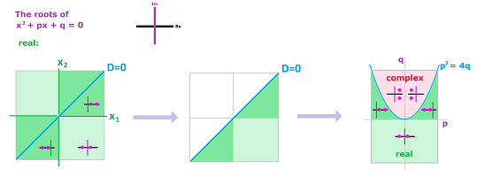
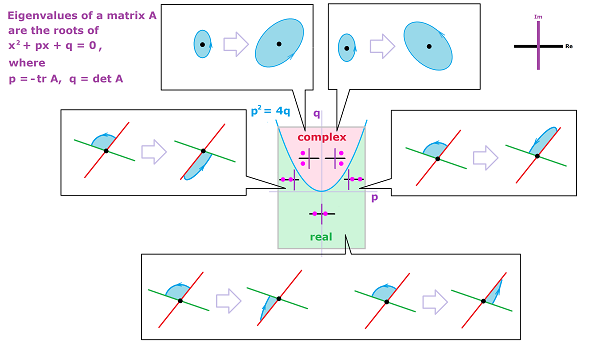
Let's visualize our conclusion. We would like to show the main scenarios of what kinds of roots the polynomial might have depending on the values of its two coefficients, $p$ and $q$.

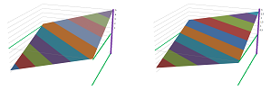
First, how do we visualize pairs of numbers? As points on a coordinate plane of course... but only when they are real. Suppose for now that they are. We start with a plane, the $x_1x_2$-plane to be exact, as a representation of all possible pairs of real roots (left). Then the diagonal of this plane represents the case of equal (and still real) roots, $x_1=x_2$, i.e., $D=0$. Since the order of the roots doesn't matter -- $(x_1,x_2)$ is as good as $(x_2,x_1)$ -- we need only half of the plane. We fold the plane along the diagonal (middle).

The diagonal -- represented by the equation $D=0$ -- exposed this way can now serve its purpose of separating the case of real and complex roots. Now, let's go to the $pq$-plane. Here, the parabola $p^2=4q$ also represents the equation $D=0$. Let's bring them together! We take our half-plane and bend its diagonal edge into the parabola $p^2=4q$ (right).

Classifying polynomials this way allows one to classify matrices and understand what each of them does as a transformation of the plane, which in turn will help us understand systems of ODEs.

The complex plane ${\bf C}$ is the Euclidean space ${\bf R}^2$

We will consider ODE of functions over complex variables. The issues we need to address in order to develop calculus of such functions are familiar from early part of this book. However, we will initially look at them through the lens of vector algebra presented in Chapter 16.

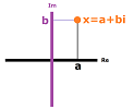
A complex number $z$ has the standard representation: $$z=a+bi,$$ where $a$ and $b$ are two real numbers. These two can be seen in the geometric representation of complex numbers:

Therefore, $a$ and $b$ are thought of as the coordinates of $z$ as a point on the plane. But any complex number is not only a point on the complex plane but also a vector. We have a one-to-one correspondence: $${\bf C}\longleftrightarrow {\bf R}^2,$$ given by $$a+bi\ \longleftrightarrow\ <a,b>.$$

There is more to this than just a match; the algebra of vectors in ${\bf R}^2$ applies!

Warning: In spite of this fundamental correspondence, we will continue to think of complex numbers as numbers (and use the lower case letters).

Let's see how this algebra of numbers works in parallel with the algebra of $2$-vectors.

First, the addition of complex numbers is done component-wise: $$\begin{array}{ll} (a+bi)&+&(c+di)&=&(a+c)&+&(b+d)i,\\ <a,b>&+&<c,d>&=&<a+c&,&b+d>. \end{array}$$

Second, we can easily multiply complex numbers by real ones: $$\begin{array}{ll} (a+bi)&c&=&(ac)&+&(bc)i,\\ <a,b>&c &=&<ac&,&bc>. \end{array}$$

Aren't complex numbers just vectors? No, not with the possibility of multiplication taken into account...

Our study of calculus of complex numbers starts with the study of the topology of the complex plane. This topology is the same as that of the Euclidean plane ${\bf R}^2$!

Just as before, every function $z=f(t)$ with an appropriate domain creates a sequence: $$z_k=f(k).$$ A function with complex values defined on a ray in the set of integers, $\{p,p+1,...\}$, is called an infinite sequence, or simply sequence with the abbreviated notation: $$z_k=\{z_k\}.$$

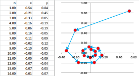
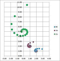
Example. A good example is that of the sequence made of the reciprocals: $$z_k=\frac{\cos k}{k}+\frac{\sin k}{k}i.$$ It tends to $0$ while spiraling around it.

$\square$

The starting point of calculus of complex numbers is the following. The convergence of a sequence of complex numbers is the convergence of its real and imaginary parts or, which is equivalent, the convergence of points (or vectors) on the complex plane seen as any plane: the distance from the $k$th point to the limit is getting smaller and smaller.

We use the definition of convergence for vectors on the plane from Chapter 16 simply replacing vectors with complex numbers and “magnitude” with “modulus”.

Definition. Suppose $\{z_k:\ k=1,2,3...\}$ is a sequence of complex numbers, i.e., points in ${\bf C}$. We say that the sequence converges to another complex number $z$, i.e., a point in ${\bf C}$, called the limit of the sequence, if: $$||z_k- z||\to 0\text{ as }k\to \infty,$$ denoted by: $$z_k\to z \text{ as }k\to \infty,$$ or $$z=\lim_{k\to \infty}z_k.$$ If a sequence has a limit, we call the sequence convergent and say that it converges; otherwise it is divergent and we say it diverges.

In other words, the points start to accumulate in smaller and smaller circles around $z$. A way to visualize a trend in a convergent sequence is to enclose the tail of the sequence in a disk:

Theorem (Uniqueness). A sequence can have only one limit (finite or infinite); i.e., if $a$ and $b$ are limits of the same sequence, then $a=b$.

Definition. We say that a sequence $z_k$ tends to infinity if the following condition holds: for each real number $R$, there exists a natural number $N$ such that, for every natural number $k > N$, we have $$||z_k|| >R;$$ we use the following notation: $$z_k\to \infty \text{ as } k\to \infty .$$

The following is another analog of a familiar theorem about the topology of the plane.

Theorem (Component-wise Convergence of Sequences). A sequence of complex numbers $z_k$ in ${\bf C}$ converges to a complex number $z$ if and only if both the real and the imaginary parts of $z_k$ converge to the real and the imaginary parts of $z$ respectively; i.e., $$z_k\to z \ \Longleftrightarrow\ \operatorname{Re}(z_k)\to \operatorname{Re}(z) \text{ and } \operatorname{Im}(z_k)\to \operatorname{Im}(z).$$

The algebraic properties of limits of sequences of complex numbers also look familiar...

Theorem (Sum Rule). If sequences $z_k ,u_k$ converge then so does $z_k + u_k$, and $$\lim_{k\to\infty} (z_k + u_k) = \lim_{k\to\infty} z_k + \lim_{k\to\infty} u_k.$$

Theorem (Constant Multiple Rule). If sequence $z_k $ converges then so does $c z_k$ for any complex $c$, and $$\lim_{k\to\infty} c\, z_k = c \cdot \lim_{k\to\infty} z_k.$$

Wouldn't calculus of complex numbers be just a copy of calculus on the plane? No, not with the possibility of multiplication taken into account.

Multiplication of complex numbers: ${\bf C}$ isn't just ${\bf R}^2$

Just like in ${\bf R}^2$, multiplication by a real number $r$ will stretch/shrink all vectors and, therefore, the complex plane ${\bf C}$. However, multiplication by a complex number $c$ will also rotate each vector.

The imaginary part of $c$ is responsible for rotation. For example, multiplication by $i$ rotates the number by $90$ degrees: $1$ becomes $i$, while $i$ becomes $-1$ etc.

How does multiplication affect topology?

Theorem (Product Rule). If sequences $z_k ,u_k$ converge then so does $z_k \cdot u_k$, and $$\lim_{k\to\infty} (z_k \cdot u_k) = \lim_{k\to\infty} z_k \cdot \lim_{k\to\infty} u_k.$$

Proof. Suppose $$z_k=a_k+b_ki\to a+bi \text{ and } u_k=p_k+q_ki=p+qi.$$ Then, according to the Component-wise Convergence Theorem above, we have: $$a_k\to a,\ b_k \to b \text{ and } p_k\to p,\ q_k\to q.$$ Then, by the Product Rule for numerical sequences, we have: $$a_kp_k\to ap,\ a_kq_k\to aq,\ b_kp_k\to bp,\ b_kq_k\to bq.$$ Then, as we know, $$z_k \cdot u_k=(a_kp_k-b_kq_k)+(a_kq_k+b_kp_k)i\to (ap-bq)+(aq+bq)i=(a+bi)(p+qi),$$ by the Sum Rule for numerical sequences. $\blacksquare$

Theorem (Quotient Rule). If sequences $z_k ,\ u_k$ converge (with $u_k\ne 0$) then so does $z_k / u_k$, and $$\lim_{k\to\infty} \frac{z_k}{ u_k} = \frac{\lim_{k\to\infty} z_k }{ \lim_{k\to\infty} u_k},$$ provided $$\lim_{k\to\infty} u_k\ne 0.$$

Just like real numbers!

Exercise. Prove the last theorem.

In addition to the standard, Cartesian, representation, a complex number $x=a+bi$ can be defined in terms of its magnitude and angle with to the $x$-axis via the polar coordinates. The former is called the modulus of $z$ denoted by: $$||z||=\sqrt{a^2+b^2}.$$ The latter is called the argument of $z$ denoted by: $$\operatorname{arg}(z)=\arctan{\frac{b}{a}}.$$

Any two real numbers $r\ge 0$ and $0\le \alpha< 2\pi$ can serve as those: $$z=r\big[ \cos \alpha+i\sin \alpha \big].$$

The algebra takes a new form too. We don't need the new representation to compute addition and multiplication by real numbers, but we need it for multiplication.

What is the product of two complex numbers: $$z_1 = r_1 \big[\cos\varphi_1 + i \sin\varphi_1\big] \text{ and } z_2 = r_2 \big[\cos\varphi_2 + i \sin\varphi_2\big]?$$ Consider: $$\begin{array}{lll} z_1z_2 &= r_1 \big[\cos\varphi_1 + i \sin\varphi_1) \big]\cdot r_2 \big[\cos\varphi_2 + i \sin\varphi_2 \big]\\ &=r_1r_2\big[ \cos\varphi_1 + i \sin\varphi_1\big]\cdot \big[\cos\varphi_2 + i \sin\varphi_2\big]\\ &=r_1r_2\big( \cos\varphi_1\cos\varphi_2 + i \sin\varphi_1\cos\varphi_2+ \cos\varphi_1\sin\varphi_2 + i^2 \sin\varphi_1\sin\varphi_2\big)\\ \end{array}$$ We utilize the following trigonometric identities $$\cos a\cos b - \sin a \sin b = \cos(a + b)$$ and $$\cos a \sin b + \sin a\cos b = \sin(a + b).$$ Then, $$z_1 z_2 = r_1 r_2 \big[ \cos(\varphi_1 + \varphi_2) + i \sin(\varphi_1 + \varphi_2) \big].$$ In other words, the modules are multiplied and the arguments are added.

Exercise. Prove that the two sequence comprised of the modulus and the argument of the terms of a sequence converge when the sequence converges.

Complex functions

A complex function is simply a function with both input and output complex numbers: $$F:{\bf C}\to{\bf C}.$$ How do we visualize these functions? The graph of a function $F$ lies in the $4$-dimensional space and isn't of much help!

To begin with, we can recast some of the transformations of the plane presented in this chapter as complex functions.

Example. The shift by vector $V=<a,b>$ becomes addition of a fixed complex number: $$F(x,y)=(x+a,y+b) \ \leadsto\ F(z)=z+z_0,$$ where $z_0=a+bi$.

$\square$

Example. The vertical flip becomes conjugation: $$F(x,y)=(x,-y)\ \leadsto\ F(z)=\bar{z}.$$

$\square$

Exercise. Find a complex formula for the horizontal flip: $$F(x,y)=(-x,y).$$

Example. The uniform stretch becomes multiplication by a real number: $$F(x,y)=(kx,ky)\ \leadsto\ F(z)=kz.$$

Of course, the flip about the origin is just multiplication by $-1$. $\square$

Exercise. Find complex formulas for the vertical stretch: $$F(x,y)=(x,ky)$$ and the horizontal stretch: $$F(x,y)=(kx,y).$$

Example. A rotation is carried out via a multiplication by a fixed complex number: $$F(z)=z_0z.$$ Specifically, it has to be a number with modulus equal to $1$: $$z_0=\cos \alpha +i\sin \alpha.$$ Meanwhile, with $z_0=2i$, we have the $90$ degrees rotation with a stretch with a factor of $2$:

$\square$

For any complex function, we represent both the independent variable and the dependent variable in terms of their real and imaginary parts, just as vector functions:

• $x = u + iv$, and
• $z = F(x) = f (u,v) + ig (u,v)$,

where $u,\ v$ are real numbers and $f(u,v),\ g(u,v)$ are real-valued functions. The two component functions, $f$ and $g$, can be plotted as well as the argument, $\operatorname {arg}F$, and the module, $||F||$.

Example. The projections on the $x$- and $y$-axes are these: $$F(z)=\operatorname{Re} z \text{ and }F(z)=\operatorname{Im} z.$$

$\square$

Example.

$\square$

Example. Let's consider a quadratic polynomial again: $$f(x)=x^2+px+q.$$ Recall that increasing the value of $q$ makes the graph of $y=f(x)$ shift upward: its two $x$-intercepts start to get closer to each other, then merge, and finally disappear:

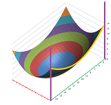
Note that an identical result is seen in a seemingly different situation. Suppose we have a paraboloid, then it produces a parabola as it is cut by a vertical plane. Suppose the paraboloid is moving horizontally. If it is fading away, the parabola is moving upward.

This illustrates what happens when our quadratic polynomial is seen as a function of a complex variable. We are plotting the real part of the function. $\square$

Warning: visualizing $F(x)$ via those functions, or as a vector field, may be misleading.

Complex functions are transformations of the complex plane!

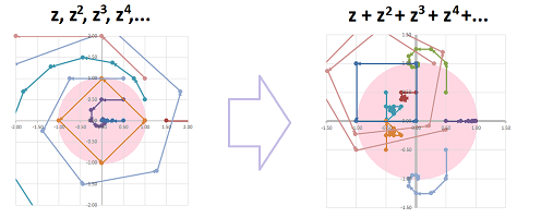
Example. This is a visualization of the power function over complex numbers. For several values of $z$, the values $$z,z^2,z^3,...$$ are plotted as sequences.

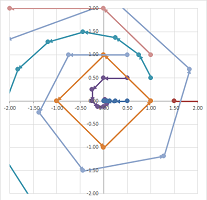
One can see how the real part of $z$ makes the multiplication by $z$ stretch or shrink the number while the imaginary part of $x$ is responsible for rotating the number around $0$. A special, square path is produced by $z=i$. $\square$

The definition is a copy of the one from Chapter 6.

Definition. The limit of a function $z=F(x)$ at a point $x=a$ is defined to be the limit $$\lim_{n\to \infty} F(x_n)$$ considered for all sequences $\{x_n\}$ within the domain of $F$ excluding $a$ that converge to $a$, $$a\ne x_n\to a \text{ as } n\to \infty,$$ when all these limits exist and are equal to each other. In that case, we use the notation: $$\lim_{x\to a} F(x).$$ Otherwise, the limit does not exist.

Theorem (Locality). Suppose two functions $f$ and $g$ coincide in the vicinity of point $a$: $$f(x)=g(x) \text{ for all }x \text{ with } ||x-a|| <\varepsilon,$$ for some $\varepsilon >0$. Then, their limits at $a$ coincide too: $$\lim_{x\to a} f(x) =\lim_{x\to a} g(x).$$

Limits under algebraic operations... We will use the algebraic properties of the limits of sequences to prove virtually identical facts about limits of functions.

Let's re-write the main algebraic properties using the alternative notation.

Theorem (Algebra of Limits of Sequences). Suppose $a_n\to a$ and $b_n\to b$. Then $$\begin{array}{|ll|ll|} \hline \text{SR: }& a_n + b_n\to a + b& \text{CMR: }& c\cdot a_n\to ca& \text{ for any complex }c\\ \text{PR: }& a_n \cdot b_n\to ab& \text{QR: }& a_n/b_n\to a/b &\text{ provided }b\ne 0\\ \hline \end{array}$$

Each property is matched by its analog for functions.

Theorem (Algebra of Limits of Functions). Suppose $f(x)\to F$ and $g(x)\to G$ as $x\to a$ . Then $$\begin{array}{|ll|ll|} \hline \text{SR: }& f(x)+g(x)\to F+G & \text{CMR: }& c\cdot f(x)\to cF& \text{ for any complex }c\\ \text{PR: }& f(x)\cdot g(x)\to FG& \text{QR: }& f(x)/g(x)\to F/G &\text{ provided }G\ne 0\\ \hline \end{array}$$

Definition. A function $f$ is called continuous at point $a$ if

• $f(x)$ is defined at $x=a$,
• the limit of $f$ exists at $a$, and
• the two are equal to each other:

$$\lim_{x\to a}f(x)=f(a).$$

Thus, the limits of continuous functions can be found by substitution.

Equivalently, a function $f$ is continuous at $a$ if $$\lim_{n\to \infty}f(x_n)=f(a),$$ for any sequence $x_n\to a$.

A typical function we encounter is continuous at every point of its domain. The most important class of continuous functions is the following.

Theorem. Every polynomial is continuous at every point.

Unlike vector functions, complex functions have more operations to worry about. The theorem follows from the following algebraic result.

Theorem (Algebra of Continuity). Suppose $f$ and $g$ are continuous at $x=a$. Then so are the following functions: $$\begin{array}{|ll|ll|} \hline \text{SR: }& f+g & \text{CMR: }& c\cdot f& \text{ for any complex }c\\ \text{PR: }& f\cdot g& \text{QR: }& f/g &\text{ provided }g(a)\ne 0\\ \hline \end{array}$$

Complex linear operators

Let's consider linear operators again. Suppose $A$ is a linear operator with a $2\times 2$ matrix with real entries. Suppose $D$ is the discriminant of the characteristic polynomial of $A$. When $D>0$, we have two distinct real roots covered by the Classification Theorem of Linear Operators with real eigenvalues. We also saw the transitional case when $D=0$. Thus, we transition to the case $D<0$ when the eigenvalues -- as roots of the characteristic polynomial -- are complex. We already know that complex numbers are just as good (or better!) than the real, so why not include this possibility?

Example. This is how we find the characteristic polynomial for the rotation and find the eigenvalues by solving it: $$A = \left[\begin{array}{} 0 & -1 \\ 1 & 0 \end{array}\right]\ \Longrightarrow\ \det \left( \left[\begin{array}{} 0 & -1 \\ 1 & 0 \end{array}\right] - \lambda \left[\begin{array}{} 1 & 0 \\ 0 & 1 \end{array}\right] \right) = \det \left[\begin{array}{} -\lambda & -1 \\ 1 & -\lambda \end{array}\right] = \lambda^2 + 1 = 0\ \Longrightarrow\ \lambda = \pm i.$$ The eigenvalues are imaginary! Let's notice though that no real vector multiplied by an imaginary number can produce a real vector... Indeed, let's try to find the eigenvectors; solve the matrix equation $AV=\lambda V$ for $V$ in ${\bf R}^2$. In other words, we need to find real(!) $x, y$ such that: $$\left[\begin{array}{} 0 & -1 \\ 1 & 0 \end{array}\right] \left[\begin{array}{} x \\ y \end{array}\right] = i \left[ \begin{array}{} x \\ y \end{array}\right]\ \Longrightarrow\ \begin{cases} -y &= ix\\ x &= iy \end{cases}.$$ Unless both zero, $x$ and $y$ can't be both real... $\square$

So, when the eigenvalues aren't real, there are no real eigenvectors.

But why stop here? Why not have all the numbers and vectors and matrices complex?

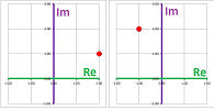
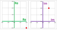
Just as a real $2$-vector is a pair of real numbers, a complex $2$-vector is a pair of complex numbers; for example, $$V=\left[\begin{array}{cc} 2&+&i \\ -1&+&2i \end{array}\right].$$ This representation is illustrated below via the real and imaginary parts of either of the two components:

Here, we see the complex plane ${\bf C}$ for the first and then the complex plane ${\bf C}$ for the second component of the vector $V$. This is why we denote the set of all complex $2$-vectors by ${\bf C}^2$.

Furthermore, this vector $V$ can be rewritten in terms of its real and imaginary parts: $$V=\left[\begin{array}{cc} 2&+&i \\ -1&+&2i \end{array}\right]=\left[\begin{array}{cc} 2 \\ -1 \end{array}\right]+i\left[\begin{array}{cc} 1 \\ 2 \end{array}\right].$$ Each of these is a real vector and they are illustrated accordingly:

The former is of the main interest and it is located in the familiar real plane ${\bf R}^2$.

Next, a complex $2\times 2$ matrix $A$ is simply a $2\times 2$ table of complex numbers; for example: $$A=\left[\begin{array}{} 0 & 1+i \\ i & 2-3i \end{array}\right].$$

The algebra of complex numbers -- addition and multiplication -- presented above allows us to carry out the operations -- addition, scalar multiplication, and matrix multiplication -- on these vectors and these matrices! Then, a complex matrix $A$ defines a function: $$A : {\bf C}^2 \to {\bf C}^2,$$ through matrix multiplication: $A(X)=AX$. Moreover, this function is a linear operator in the following sense: $$A(\alpha X+\beta Y)=\alpha A(X)+\beta A(Y),$$ for any complex numbers $\alpha$ and $\beta$ and any complex vectors $X$ and $Y$.

But how can we use these functions to understand real linear operators? Its inputs and outputs are complex vectors and they have real parts as discussed above. So, we can restrict the domain of a complex linear operator to the real plane first and then take the real part of the output. The result is a familiar real linear operator: $$B : {\bf R}^2 \to {\bf R}^2,$$ the real part of the complex linear operator $A$.

Let's review our theory generalized this way.

Definition. The determinant of a complex $2\times 2$ matrix is defined to be the following complex number: $$\det \left[\begin{array}{} a & b \\ c & d \end{array}\right]=ad-bc.$$

Theorem. Suppose $A$ is a complex $2\times 2$ matrix. Then, $\det A\ne 0$ if and only if the solution set of the matrix equation $AX=0$ consists of only $0$.

Definition. Given a linear operator $A : {\bf C}^2 \to {\bf C}^2$, a (complex) number $\lambda$ is called an eigenvalue of $A$ if $$A(V)=\lambda V,$$ for some non-zero vector $V$ in ${\bf C}^2$. Then, $V$ is called an eigenvector of $A$ corresponding to $\lambda$.

Definition. For a (complex) eigenvalue $\lambda$ of $A$, the eigenspace of a complex linear operator $A$ corresponding to $\lambda$ is defined and denoted by the following set in ${\bf C}^2$: $$E(\lambda) = \{ V :\ A(V)=\lambda V \}.$$

It is a very important fact that all the computations that we have performed on real matrices and vectors remain valid! Among the results that remain valid is the Classification of Linear Operators with real eigenvalues.

Linear operators represented by real matrices however will remain our exclusive interest.

Every linear operator represented by a real matrix $A$ is still just a special case of a complex operator $A : {\bf C}^2 \to {\bf C}^2$. In fact, it will always have some complex (non-real) vectors among its values, unless $A=0$. Its characteristic polynomial has real coefficients and, therefore, the Classification Theorem of Quadratic Polynomials presented in this chapter applies, as follows.

Theorem (Classification Theorem of Eigenvalues). Suppose $A$ is a linear operator represented by a real $2\times 2$ matrix $A$ and $D$ is the discriminant of its characteristic polynomial. Then the eigenvalues $\lambda_1,\ \lambda_2$ of $A$ fall into one of the following three categories:

• if $D>0$, then $\lambda_1,\ \lambda_2$ are distinct real;
• if $D=0$, then $\lambda_1,\ \lambda_2$ are equal real;
• if $D<0$, then $\lambda_1,\ \lambda_2$ are complex conjugate.

We only need to address the last case.

Linear operators with complex eigenvalues

All numbers below are complex unless stated otherwise.

The first thing we notice about the case when the eigenvalues of a linear operator aren't real is that there are no real eigenvectors. There will be no eigenspaces shown in the real plane shown in the examples below.

Example (rotations). Consider a rotation through $90$ degrees counterclockwise again: $$\left[ \begin{array}{} u \\ v \end{array}\right] = \left[\begin{array}{} 0&-1\\1&0 \end{array} \right] \, \left[ \begin{array}{} x \\ y \end{array} \right]\ \Longrightarrow\ \lambda_{1,2}=\pm i.$$

To find the first eigenvector, we solve: $$FV_1=\left[ \begin{array}{ccc} 0&-1\\ 1&0 \end{array}\right]\left[\begin{array}{cc} x\\ y \end{array}\right]=i\left[\begin{array}{cc} x\\ y \end{array}\right].$$ This gives as the following system of linear equations: $$\begin{cases} &-y&=ix\\ x&&=iy \end{cases} \ \Longrightarrow\ y=-ix.$$ We choose a complex eigenvector: $$V_1=\left[\begin{array}{cc} 1\\ -i \end{array}\right],$$ and similarly an eigenvector for the second eigenvalue: $$V_2=\left[\begin{array}{cc} 1\\ i \end{array}\right].$$ The rest are (complex) multiples of these.

So, under $F$, complex vector $V_k$ is multiplied by $\lambda_k$, and so is every of its multiples, $k=1,2$. Since these multiples are complex, this multiplication rotates (the vector of the geometric representation of) either component of this vector. Furthermore, the real part of this vector is also rotated -- on the real plane. It is this rotation that we are interested in. It is shown in the second row below:

The general value is a linear combination -- over the complex numbers -- of our two eigenvectors: $$X=\alpha \, V_1+\beta\, V_2\ \Longrightarrow\ FX =\alpha i\left[\begin{array}{cc}1\\-i\end{array}\right]+\beta(-i)\left[\begin{array}{cc}1\\i\end{array}\right].$$ $\square$

Let's consider a rotation through an arbitrary angle $\theta$: $$\left[\begin{array}{} u \\ v \end{array}\right] = \left[\begin{array}{rrr} \cos \theta & -\sin \theta \\ \sin \theta & \cos \theta \end{array} \right] \, \left[\begin{array}{} x \\ y \end{array}\right].$$

Then, we have $$\chi_A(\lambda)=(\cos\theta-\lambda)^2+\sin^2\theta =\cos^2\theta-2\cos\theta\,\lambda+\lambda^2+\sin^2\theta =\lambda^2-2\cos\theta\,\lambda+1.$$ Therefore, $$\lambda_{1,2}=\frac{2\cos\theta \pm \sqrt{(2\cos\theta)^2-4}}{2} =\frac{2\cos\theta \pm 2\sqrt{\cos^2\theta-1}}{2} =\cos\theta \pm \sqrt{-\sin^2\theta} =cos\theta \pm i\sin\theta.$$ So, the argument of the complex eigenvalues is equal to the angle of rotation (up to a sign): $$|\operatorname{arg}\lambda_{1,2}|=|\theta|.$$ The eigenvectors are the same as in the last example: $$V_1=\left[\begin{array}{cc}1\\-i\end{array}\right] \text{ and }V_2=\left[\begin{array}{cc}1\\i\end{array}\right].$$ Indeed, they are rotated through multiplication by the eigenvalues: $$\lambda_k V_k=(cos\theta \pm i\sin\theta)\left[\begin{array}{cc} 1\\ \mp i \end{array}\right] =\left[\begin{array}{cc} \cos\theta \pm i\sin\theta\\ \sin\theta \mp i\cos\theta \end{array}\right]=\left[\begin{array}{rrr} \cos \theta & -\sin \theta \\ \sin \theta & \cos \theta \end{array}\right]\left[\begin{array}{cc} 1\\ \mp i \end{array}\right].$$

Once again, we see how the real part of a complex eigenvector is rotated via complex multiplication:

Warning: this does not apply to vector in ${\bf C}^2$ that aren't eigenvectors.

Example (rotation with stretch-shrink). Let's consider this linear operator: $$\begin{cases} u&=3x&-13y,\\ v&=5x&+y\end{cases} \text{ and }F=\left[ \begin{array}{cc} 3&-13\\ 5&1 \end{array}\right].$$

Our analysis starts with the characteristic polynomial: $$\chi(\lambda)=\det (F-\lambda I)=\det \left[ \begin{array}{cc}3-\lambda&-13\\5&1-\lambda\end{array}\right]=\lambda^2-4\lambda+68.$$ We find the eigenvalues from the Quadratic Formula: $$\lambda_{1,2}=2\pm 8i.$$

Now we find the eigenvectors. We solve the two equations: $$FV_k=\lambda_k V_k,\ k=1,2.$$ The first: $$FV_1=\left[ \begin{array}{cc} 3&-13\\ 5&1 \end{array}\right]\left[\begin{array}{cc} x\\ y \end{array}\right]=(2+8i)\left[\begin{array}{cc} x\\ y \end{array}\right].$$ This gives as the following system of linear equations: $$\begin{cases} 3x&-13y&=(2+8i)x\\ 5x&+y&=(2+8i)y \end{cases} \ \Longrightarrow\ \begin{cases} (1-8i)x&-13y&=0\\ 5x&+(-1-8i)y&=0 \end{cases} \ \Longrightarrow\ x=\frac{(1+8i)}{5}y.$$ We choose the first eigenvector to be: $$V_1=\left[\begin{array}{cc} 1+8i\\ 5 \end{array}\right].$$

The second eigenvalue satisfies: $$FV_2=\left[ \begin{array}{cc} 3&-13\\ 5&1 \end{array}\right]\left[\begin{array}{cc} x\\ y \end{array}\right]=(2- 8i)\left[\begin{array}{cc} x\\ y \end{array}\right].$$ We have the following system: $$\begin{cases} 3x&-13y&=(2-8i)x\\ 5x&+y&=(2-8i)y \end{cases} \ \Longrightarrow\ \begin{cases} (1+8i)x&-13y&=0\\ 5x&+(-1+8i)y&=0 \end{cases}\ \Longrightarrow\ x=\frac{(1-8i)}{5}y.$$ We choose the second eigenvector to be: $$V_2=\left[\begin{array}{cc} 1-8i\\ 5 \end{array}\right].$$

The general complex value is a linear combination of the two: $$X=\alpha\, V_1+\beta\, V_2\ \Longrightarrow\ FX=\alpha(2+8i)\left[\begin{array}{cc}1+8i\\5\end{array}\right]+\beta(2-8i)\left[\begin{array}{cc}1-8i\\5\end{array}\right].$$

We know the effect of $F$ on these two vectors: they are rotated and stretched.

As you can see, stretching is the same for both components and both basis vectors. That is why we have -- in addition to the rotation -- a uniform stretch (re-scaling) for the real plane. This is shown in the second row.

This is the algebra for the above illustration: $$\lambda_1V_1=(2+8i)\left[\begin{array}{cc}1+8i\\5\end{array}\right]=\left[\begin{array}{cc}-62+24i\\10+40i\end{array}\right] \text{ and } \lambda_2V_2=(2-8i)\left[\begin{array}{cc}1-8i\\5\end{array}\right]=\left[\begin{array}{cc}-62-24i\\10-40i\end{array}\right].$$ $\square$

According to the Classification Theorem of Quadratic Polynomials, when the discriminant $D<0$, the two roots are conjugate: $$\lambda_{1,2}=a\pm bi.$$ They have the same modulus: $$||\lambda_{1,2}||=\sqrt{a^2+ b^2}.$$ This is why multiplying any complex number by either of the two numbers will produce the same rate of stretch. We conclude that ${\bf C}^2$ and, especially, the real plane ${\bf R}^2$ are stretched uniformly! This is the summary of our analysis.

Theorem (Classification of linear operators with complex eigenvalues). Suppose a real matrix $F$ has two complex conjugate eigenvalues $\lambda_1$ and $\lambda_2$. Then, the operator $U=FX$

• 1. rotates the real plane through the angle $\theta$ that satisfies the following:

$$|\sin\theta|=|\operatorname{arg} \lambda_1|=|\operatorname{arg} \lambda_2|,$$

• 2. stretches-shrinks the plane uniformly by the following factor:

$$s=||\lambda_1||=||\lambda_2||.$$

We can also recast this theorem in exclusively “real” terms.

We will need to the following result.

Theorem. If a quadratic polynomial, $$x^2+px+q,$$ has a non-positive discriminant, $$D=p^2-4q \le 0,$$ then either of its roots, $$x=\frac{1}{2}(-p \pm \sqrt{D} ),$$ has its argument satisfy: $$\sin\big( \operatorname{arg}x \big)=\frac{1}{2}\sqrt{ 4-\frac{p^2}{q} },$$ and its module satisfy: $$||x||^2=q.$$

Proof. The modulus of the roots is the following: $$||x||^2=\big(\operatorname{Re}x\big)^2+\big(\operatorname{Im}x\big)^2=\frac{1}{4}( p^2 + |D| )=\frac{1}{4}( p^2 -D )=\frac{1}{4}\big( p^2 -( p^2-4q )\big)=q.$$ And their argument satisfies the following: $$\sin\big( \operatorname{arg}x \big)=\frac{ \operatorname{Im}x} {||x||}=\frac{ \frac{1}{2}\sqrt{D} } { \sqrt{q} }=\frac{1}{2}\sqrt{ \frac{-D}{q} }=\frac{1}{2}\sqrt{ -\frac{p^2-4q}{q} }=\frac{1}{2}\sqrt{ 4-\frac{p^2}{q} }.$$ $\blacksquare$

We define the trace of a matrix as the sum of its diagonal elements: $$\operatorname{tr}\left[ \begin{array}{ll}a&b\\c&d\end{array}\right]=a+d.$$ Then the characteristic polynomial takes this form: $$\begin{array}{lll} \chi(\lambda)&=\det\left[ \begin{array}{cc} a-\lambda & b \\ c & d-\lambda \end{array}\right]\\ &=ad-a\lambda-\lambda d+\lambda^2 -bc\\ &=\lambda^2-(a+d)\lambda+(ad-bc)\\ &=\lambda^2-\operatorname{tr} F\,\lambda+\det F.\\ \end{array}$$ We match this to the theorem above: $$p=-\operatorname{tr} F,\ q=\det F,\ D=(\operatorname{tr} F)^2-4\det F.$$ The roots are $$\lambda_{1,2}=\frac{1}{2}\big(\operatorname{tr} F \pm \sqrt{D} \big).$$ When the roots are complex, the modulus is the following: $$||\lambda_{1,2}||=\sqrt{\det F }.$$ And their argument satisfies the following: $$\sin\big( \operatorname{arg}\lambda_{1,2} \big)=\frac{1}{2} \sqrt{ \frac{(\operatorname{tr} F)^2}{\det F} -4 }.$$

This is the final result.

Corollary. Suppose a real matrix $F$ satisfies: $$D=(\operatorname{tr} F)^2-4\det F \le 0.$$ Then, the operator $U=FX$

• 1. rotates the real plane through the following angle:

$$\theta=\sin^{-1}\left( \frac{1}{2}\sqrt{ \frac{4-(\operatorname{tr} F)^2}{\det F} } \right);$$

• 2. stretches-shrinks the plane uniformly by the following factor:

$$s=\sqrt{\det F }.$$

Yes, we have included the transitional case $D=0$! Indeed, it has the same stretch but no rotation.

We finally put together our two classification theorems: the behavior of linear operators in terms of the eigenvalues -- real or complex -- of their matrices. We illustrate this classification below in the context of the Classification of Roots of Quadratic Polynomials:

Complex calculus

In spite of the representation of complex numbers by plane vectors, the formula for the derivative of a complex function doesn't follow the idea of the gradient but rather follows, and is identical to, the definition of the derivative of a real function. We rely on the fact that the algebra is the same even though the numbers are different.

Definition. The derivative of a complex function $u=f(x)$ at $x=a$ is defined to be the limit of the difference quotients at $x=a$ as the increment $\Delta x$ is approaching $0$, denoted by: $$f'(x)=\lim_{x\to a}\frac{f(x)-f(a)}{x-a}=\lim_{||x-a||\to 0}\frac{f(x)-f(a)}{x-a};$$ in that case the function is called differentiable at $x=a$.

This formula is made possible by the availability of multiplication and division.

Warning: The formula is not the same as this: $$\lim_{x\to a}\frac{f(x)-f(a)}{||x-a||}.$$

Warning: The idea of the derivative isn't about the slope, rise over the run, anymore.

The derivative is still the instantaneous rate of change of the output relative to the input.

Many result are familiar such as the following.

Theorem. If a function is differentiable, it is also continuous.

Example. Computations work out in the exactly the same manner. Let's compute $f'(2)$ from the definition for $$f(x) = -x^{2} - x. $$ Definition: $$f'(2) = \lim_{h \to 0} \frac{f(2 + h) - f(2)}{h}. $$ To compute the difference quotient, we need to substitute twice: $$f(2 + h) = -(2 + h)^{2} - (2 + h),\ f(2) = -2^{2} - 2.$$ Now, we substitute into the definition: $$\begin{aligned} f'(2) &= \lim_{h \to 0} \frac{\left[ -(2 - h)^{2} - (2-h) \right] - \left[ -2^{2} - 2 \right]}{h} \\ &= \lim_{h \to 0} \frac{-4 - 4h - h^{2} - 2 - h + 4 + 2}{h} \\ &= \lim_{h \to 0} \frac{-5h - h^{2}}{h} \\ &= \lim_{h \to 0} (-5 -h ) \\ &= -5 - 0 \\ &= 5. \end{aligned}$$ $\square$

Theorem (Integer Power Formula). The derivative of $x^n$ is given by $$\begin{array}{ll} (x^n)'= n x^{n - 1}\\ \end{array}$$

Proof. The proof relies entirely on the formula: $$a^n-b^n=(a-b)(a^{n-1}+a^{n-2}b+...+ab^{n-2}+b^{n-1}).$$ $\blacksquare$

There is a counterpart for each rule of differentiation!

Theorem (Algebra of Derivatives). Wherever complex functions $f$ and $g$ are differentiable, we have the following: $$\begin{array}{|ll|ll|} \hline \text{SR: }& (f+g)'=f'+g' & \text{CMR: }& (cf)'=cf'& \text{ for any complex }c\\ \text{PR: }& (fg)'=f'g+fg'& \text{QR: }& (f/g)'=\frac{f'g-fg'}{g^2} &\text{ provided }g\ne 0\\ \hline \end{array}$$

We can differentiate any polynomial easily now.

Theorem. For any positive integer $n$ and any complex numbers $a_0,...,a_n$, we have the following: $$\begin{array}{lllll} &\big(a_nx^{n} + & a_{n-1}x^{n-1}& + a_{n-2}x^{n-2} &+...&+ a_2x^2&+a_1x&+a_0\big)'\\ =&a_nnx^{n-1} + & a_{n-1}(n-1)x^{n-2}& + a_{n-2}(n-2)x^{n-3} &+...&+ a_22x&+a_1&&. \end{array}$$

As far as applications are concerned, there is no such a relation as “less” or “more” among complex numbers! That's why we don't have to worry about:

• monotonicity,
• extreme points,
• concavity, etc.

Just as before, reversing differentiation is called integration and the resulting functions are called antiderivatives; $F$ is an antiderivative of $f$ if $F'=f$.

There is a counterpart for each rule of integration!

Theorem (Algebra of Anti-Derivatives). Wherever $f$ and $g$ are integrable, we have the following: $$\begin{array}{|ll|ll|} \hline \text{SR: }& \int (f+g)\, dx=\int f\, dx+\int g\, dx & \text{CMR: }& \int (cf)\, dx=c\int f\, dx& \text{ for any complex }c\\ \text{PR: }& \int f\, dg=fg-\int g\, df& \text{LCR: }& \int f(mx+b)\, dx=\tfrac{1}{m}\int f(t)\, dt\Big|_{t=mx+b} &\text{ provided }m\ne 0\\ \hline \end{array}$$

Series and power series

All the definitions and theorems continue to be identical or virtually identical to the ones in Chapter 15.

Definition. For a given sequence $\{z_n\}=\{z_n:\ n=s,s+1,s+2,...\}$ of complex numbers, its sequence of partial sums $\{p_n:\ n=s,s+1,s+2,...\}$ is a sequence defined by the following recursive formula: $$p_s=z_s,\quad p_{n+1}=p_n+z_n,\ n=s,s+1,s+2,....$$

Definition. For a sequence $\{z_n\}$, the limit $S$ of its sequence of partial sums $\{p_n\}$ is called by the sum of the sequence or, more commonly, the sum of the series, denoted by: $$S=\sum_{i=s}^\infty z_i=\lim_{n \to \infty} \sum_{i=s}^n z_i.$$

This limit might also be infinite.

From the Uniqueness of Limit we derive the following.

Theorem (Uniqueness of Sum). A series can have only one limit (finite or infinite); i.e., if $a$ and $b$ are sums of the same series, then $a=b$.

From the Component-wise Convergence of Sequences we derive the following.

Theorem (Component-wise Convergence of Series). A series of complex numbers $\sum_{i=s}^\infty z_i$ i converges to a complex number $z$ if and only if both the real and the imaginary parts of the sequence of partial sums of $z_k$ converge to the real and the imaginary parts of $z$ respectively; i.e., $$\sum_{i=s}^\infty z_i= z \ \Longleftrightarrow\ \operatorname{Re}\sum_{i=s}^\infty z_i= \operatorname{Re}(z) \text{ and } \operatorname{Im}\sum_{i=s}^\infty z_i= \operatorname{Im}(z).$$

Example.

Definition. For a sequence $\{z_n\}$, the series: $$\sum_{i=\infty}^n z_i,$$ converges absolutely if the series of its moduli, $$\sum_{i=\infty}^n ||z_i||,$$ converges.

Example.

Now, the algebra of series.

Just as before, we can multiply a convergent series by a number term by term.

Theorem (Constant Multiple Rule for Series). Suppose $\{s_n\}$ is a sequence. For any integer $a$ and any complex $c$, we have: $$ \sum_{a}^{\infty} (c\cdot s_n) = c \cdot \sum_{a}^{\infty} s_n,$$ provided the series converges.

Just as before, we can add two convergent series term by term.

Theorem (Sum Rule for Series). Suppose $\{s_n\}$ and $\{t_n\}$ are sequences. For any integer $a$, we have: $$\sum_{a}^{\infty} \left( s_n + t_n \right) = \sum_{a}^{\infty} s_n + \sum_{a}^{\infty} t_n, $$ provided the two series converge.

Exercise. Prove these theorems.

Definition. The series produced by the geometric progression $a_n=a\cdot r^n$ with ratio $r$ (a complex number), $$\sum_{n=s}^\infty ar^n=ar^1+ar^2+ar^3+ar^4+...+ar^n+...,$$ is called the geometric series with ratio $r$.

Its sum is found the same way as for real variable.

Theorem (Sum of Geometric Series). The geometric series with ratio $r$ converges absolutely when $||r||<1$ and diverges when $||r||>1$. In the former case, the sum is: $$\sum_{n=0}^\infty ar^n=\frac{a}{1-r}.$$

The only difference is that the absolute value is replaced with the modulus.

Example. This is a visualization of a power series over complex numbers. We consider the series: $$z+z^2+z^3+...$$ For several values of $z$, the sequence and then the partial sums of the series are plotted. We can see how starting from a point inside the disk $||z||\le 1$ produces divergence and outside produces divergence:

Indeed, the series $$1+z+z^2+z^3+...$$ is a geometric series with the ratio $r=z$. Therefore, it converges for all $||z||<1$, according to the theorem, and diverges for all $||z||>1$. In other words, it converges on the disk of radius $1$ centered at $0$ in ${\bf C}$ and diverges outside of it. This circle is the domain of the function defined by the series. We even have a formula for this function: $$1+z+z^2+z^3+..=\frac{1}{1-z}.$$ The difference between the two is in the domain. $\square$

Example. There is a hint at the idea of complex power series in Chapter 16. Let's compare the Taylor series of sine, cosine and the exponential function. The sine is odd and its Taylor series only includes odd terms: $$\sin x=\sum_{k=0}^\infty \frac{(-1)^k}{(2k+1)!}x^{2k+1}.$$ The cosine is even and its Taylor series only includes even terms: $$\cos x=\sum_{k=0}^\infty \frac{(-1)^k}{(2k)!}x^{2k}.$$ If we write them one under the other, we see how they complement each other: $$\begin{array}{r|ccc} n&0&1&2&3&4&5&...\\ \hline \sin x&&x&&-\frac{x^3}{3!}&&\frac{x^5}{5!}&...\\ \cos x&1&&-\frac{x^2}{2!}&&\frac{x^4}{4!}&&... \end{array}$$ What if we add the exponential function to this? $$\begin{array}{r|cccccccc} n&0&1&2&3&4&5&...\\ \hline \sin x&0&x&0&-\frac{x^3}{3!}&0&\frac{x^5}{5!}&...\\ \cos x&1&0&-\frac{x^2}{2!}&0&\frac{x^4}{4!}&0&...\\ \hline e^x&1&x&\frac{x^2}{2!}&\frac{x^3}{3!}&\frac{x^4}{4!}&\frac{x^5}{5!}&... \end{array}$$ This looks almost like addition!.. except for those minus signs. That's where $i$ comes in. Let's substitute $x=it$: $$\begin{align} e^{it} &{}= 1 + it + \frac{(it)^2}{2!} + \frac{(it)^3}{3!} + \frac{(it)^4}{4!} + \frac{(it)^5}{5!} + \cdots \\[8pt] &{}= 1 + it - \frac{t^2}{2!} - \frac{it^3}{3!} + \frac{t^4}{4!} + \frac{it^5}{5!} - \cdots \\[8pt] &{}= \left( 1 - \frac{t^2}{2!} + \frac{t^4}{4!} - \cdots \right) + i\left( t - \frac{t^3}{3!} + \frac{x^5}{5!} - \cdots \right) \\[8pt] &{}= \cos t + i\sin t . \end{align}$$ $\square$

It is called Euler's formula. More general is the following: $$e^{a+bi} = e^a(\cos b + i\sin b) .$$ In complex calculus, functions are more interrelated!

Exercise. Show that $\sin^2 x+\cos^2 x=1$.

Definition. A sequence $\{q_n\}$ of polynomials given by a recursive formula: $$q_{k+1}(x)=q_k(x)+c_{k+1}(x-a)^{k+1},\ k=0,1,2,...,$$ for some fixed (complex) number $a$ and a sequence of (complex) numbers $\{c_k\}$, is called a power series centered at $a$. The function represented by the limit of $q_n$ is called the sum of the series, written as: $$f(x)=c_0+c_1(x-a)+c_2(x-a)^2+...=\sum_k c_k(x-a)^k=\lim_{k\to \infty} q_k(x),$$ for all $x$ for which the limit exists.

Then the three power series in the example above may serve as definitions of these three functions of complex variable: $$\begin{array}{r|cccccccc} n&0&1&2&3&4&5&&...\\ \hline \sin x=&&x&&-\frac{x^3}{3!}&&+\frac{x^5}{5!}&+&...\\ \cos x=&1&&-\frac{x^2}{2!}&&+\frac{x^4}{4!}&&-&...\\ e^x=&1&+x&+\frac{x^2}{2!}&+\frac{x^3}{3!}&+\frac{x^4}{4!}&+\frac{x^5}{5!}&+&..., \end{array}$$ pending the proof of their convergence.

We will accept the following without proof.

Theorem (The Weierstrass M-Test). Consider the power series $$\sum_{n=0}^{\infty} c_n(z−a)^n.$$ If there exists a sequence of non-negative real numbers $\{M_n\}$ such that $$|c_n(z−a)^n|\le M_n,\ n=0,1,2,...,$$ for all $z$ in an open disk $D$ around $a$ and such that the series $\sum_{n=0}^{\infty}M_n$ (of real numbers) converges. Then the power series converges uniformly on $D$.

Convergence of the three series above follows.

Definition. The greatest lower bound $r$ (that could be infinite) of the distances from $a$ to a point for which a power series centered at $a$ diverges is called the radius of convergence of the series.

This definition is legitimate according to the Existence of $\sup$ Theorem from Chapter 5.

We finally can see where the word “radius” comes from.

Theorem. Suppose $r$ is the radius of convergence of a power series $$\sum_{n=0}^\infty c_n(x-a)^n.$$ Then,

• 1. when $r<\infty$, the domain of the series is a disk $B(a,R)$ in ${\bf C}$ of radius $r$ centered at $a$ with some points on its boundary possibly included, and
• 2. when $r=\infty$, the domain of the series is the whole ${\bf C}$.

Example. $$\begin{array}{ll|c} \text{series}&\text{sum}&\text{domain}\\ \hline \sum_{k=0}^\infty x^k&=\frac{1}{1-x}&B(0,1)\\ \sum_{k=0}^\infty \frac{(-1)^k}{k!}x^k&=e^x&{\bf C}\\ \sum_{k=0}^\infty \frac{(-1)^k}{(2k+1)!}x^{2k+1}&=\sin x&{\bf C}\\ \sum_{k=0}^\infty \frac{(-1)^k}{(2k)!}x^{2k}&=\cos x&{\bf C} \end{array}$$ $\square$

Solving ODEs with power series

Recall from Chapter 16 the following important results.

Theorem (Uniqueness of Power Series). If two power series are equal, as functions, on an open interval $(a-r,a+r),\ r>0$, then their corresponding coefficients are equal, i.e., $$\sum_{n=0}^{\infty} c_n(x-a)^n=\sum_{n=0}^{\infty} d_n(x-a)^n \text{ for all } a-r<x<a+r\ \Longrightarrow\ c_n=d_n \text{ for all } n=0,1,2,3...$$

Theorem (Term-by-Term Differentiation and Integration). Suppose $R>0$ is the radius of convergence of a power series $$f(x)=\sum_{n=0}^{\infty} a_n(x-a)^n.$$ Then the function $f$ represented by this power series is differentiable (and, therefore, integrable) on the open disk $|x-a|<R$ and the power series representations of its derivative and its antiderivative converge on this disk and are found by term by term differentiation and integration of the power series of $f$, i.e., $$f'(x)=\left( \sum_{n=0}^{\infty} c_n(x-a)^n \right)'=\sum_{n=0}^{\infty} \left( c_n(x-a)^n \right)'=\sum_{n=1}^{\infty} nc_n(x-a)^{n-1},$$ and $$\int f(x)\, dx=\int \left(\sum_{n=0}^{\infty} c_n(x-a)^n\right)\, dx=\sum_{n=0}^{\infty} \int c_n(x-a)^n\, dx= \sum_{n=0}^{\infty} \frac{c_n}{n+1}(x-a)^{n+1}.$$

Example (ODEs of first order). Suppose we need to solve this initial value problem (we pretend we don't know the answer): $$y'=ky, \ y(0)=y_0.$$ The solution is the same as the one presented in Chapter 16. We assume that the unknown function $y=y(x)$ is differentiable and, therefore, is represented by a term-by-term differentiable power series.

We differentiate the series and then match the terms according to the equation: $$\begin{array}{ccc} y&=&c_0&+&c_1x&+&c_2x^2&+&c_3x^3&+&...&+&c_nx^n&+&...\\ y'&=&\ &&c_1&+&2c_2x&+&3c_3x^2&+&...&+&nc_nx^{n-1}&+&...\\ \Longrightarrow&&&\swarrow&&\swarrow&&\swarrow&&...&&\swarrow&&\\ y'&=&c_1&+&2c_2x&+&3c_3x^2&+&...&+&nc_nx^{n-1}&+&(n+1)c_{n+1}x^{n}&+...\\ ||&&||&&||&&||&&&&||&&||\\ k\cdot y&=&kc_0&+&kc_1x&+&kc_2x^2&+&...&+&kc_{n-1}x^{n-1}&+&kc_{n}x^n&+...\\ \end{array}$$ According to the Uniqueness of Power Series, the coefficients have to match! Thus, we have a sequence of equations: $$\begin{array}{ccccc} &c_1&2c_2&3c_3&...&(n+1)c_{n+1}&+...\\ &||&||&||&&||\\ &kc_0&kc_1&kc_2&...&kc_n&+...\\ \end{array}$$

We can start solving these equations from left to right: $$\begin{array}{llllllll} &c_1&\Longrightarrow\ c_1=kc_0 & &2c_2&\Longrightarrow\ c_2=k^2c_0/2& &3c_3&...\\ &||&&&||&&&||&&\\ &kc_0& &\Longrightarrow&kc_1=k^2c_0& &\Longrightarrow&kc_2=k^3c_0/2&...\\ \end{array}$$ The condition $y(0)=y_0$ means that $c_0=y_0$. Therefore, $$c_n=y_0\frac{k^n}{n!}.$$ We recognize the resulting series: $$y=\sum_{n=0}^\infty y_0\frac{k^n}{n!}x^n=y_0\sum_{n=0}^\infty \frac{1}{n!}(kx)^n=y_0e^{kx}.$$

Note to get the $n$th term we solve a system of linear equations with the following the augmented matrix: $$\left[ \begin{array}{cccccccc|c} k&-1&0&0&0&...&0&0&0\\ 0&k&-2&0&0&...&0&0&0\\ 0&0&k&-3&0&...&0&0&0\\ ...&...&...&...&...&...&...&...&...\\ 0&0&0&0&0&...&k&-n&0\\ \end{array}\right].$$ $\square$

Warning: recognizing the resulting series isn't to be expected.

Exercise. Solve the initial value problem: $$y'=ky+1, \ y(0)=y_0.$$

Example (ODEs of second order). Suppose we need to solve this initial value problem: $$y' '=-y, \ y(0)=y_0, \ y'(0)=v_0.$$ Again, we assume that the unknown function $y=y(x)$ is represented by a term-by-term differentiable power series.

We differentiate the series twice and then match the terms according to the equation: $$\begin{array}{ccccc} y&=&c_0&+&c_1x&+&c_2x^2&+&c_3x^3&+&c_4x^4&+&c_5x^5&+&...\\ y'&=&\ &&c_1&+&2c_2x&+&3c_3x^2&+&4c_nx^{3}&+&5c_nx^{4}&+&...\\ y' '&=&\ &&\ &+&2c_2&+&3\cdot 2c_3x&+&4\cdot 3c_nx^{2}&+&5\cdot 4c_nx^{3}&+&...\\ \Longrightarrow\\ y' '&=&2c_2&+&3\cdot 2c_3x&+&4\cdot 3c_4x^{2}&+&5\cdot 4c_nx^{3}&+&...\\ ||&&||&&||&&||&&&&\\ -y&=&-c_0&+&-c_1x&+&-c_2x^2&+&-c_3x^3&+&...\\ \end{array}$$ The coefficients have to match: $$\begin{array}{ccccc} &2c_2&3\cdot 2c_3&4\cdot 3c_4&5\cdot 4c_5&...&n(n-1)c_n&...\\ &||&||&||&||\\ &-c_0&-c_1&-c_2&-c_3&...&-c_{n-2}&...\\ \end{array}$$

We can start solving these equations from left to right, odd separate from even. First, for even $n$: $$\begin{array}{rlllllll} &2c_2&\Longrightarrow\ c_2=c_0/2 & &4\cdot 3c_4&\Longrightarrow\ c_4=-c_0/(4\cdot 3\cdot 2)& ...\Longrightarrow &c_n=\pm c_0/n!&...\\ &||&&&||&&&\\ &-c_0& &\Longrightarrow&-c_2=-c_0/2& &\\ \end{array}$$ The condition $y(0)=y_0$ means that $c_0=y_0$. Therefore, $$n\text{ even }\Longrightarrow\ c_n=(-1)^{n/2+1} \frac{y_0}{n!}.$$ We recognize the resulting series: $$\sum_{\text{ even }n=0}^\infty (-1)^{n/2+1} \frac{y_0}{n!}x^n =y_0\sum_{\text{ even }n=0}^\infty (-1)^{n/2+1} \frac{1}{n!}x^n= y_0\cos x .$$

Second, for odd $n$: $$\begin{array}{rlllllll} &3\cdot 2c_3&\Longrightarrow\ c_3=c_1/(3\cdot 2) & &5\cdot 4c_5&\Longrightarrow\ c_5=-c_1/(5\cdot 4\cdot 3\cdot 2)&... &\Longrightarrow &c_n=\pm c_1/n!&...\\ &||&&&||&&&\\ &-c_1& &\Longrightarrow&-c_3=-c_1/(3\cdot 2)& \\ \end{array}$$ The condition $y'(0)=v_0$ means that $c_1=v_0$. Therefore, $$n\text{ odd }\Longrightarrow\ c_n=(-1)^{(n+1)/2} \frac{v_0}{n!}.$$ We recognize the resulting series: $$y=\sum_{\text{ odd }n=1}^\infty (-1)^{(n+1)/2} \frac{v_0}{n!}x^n=v_0\sum_{\text{ odd }n=1}^\infty (-1)^{(n+1)/2} \frac{1}{n!}x^n=v_0\sin x.$$

This is the result: $$y=y_0\cos x+v_0\sin x.$$ $\square$

Exercise. Provide the augmented matrix for this system of linear equations.

Exercise. Solve the initial value problem: $$y' '+xy'+y=0, \ y(0)=1, \ y'(0)=1.$$

Example. Now let's consider something less recognizable....

$\square$

When the resulting series isn't recognizable, it is used to approximate the answer via its partial sums. The accuracy of this approximation is given by the error bound for Taylor polynomials given in Chapter 16, as follows.

Theorem (Error bound). Suppose a function $y=y(x)$ is $(n+1)$ times differentiable at $x=a$. Suppose also that for each $i=0,1,2,...,n+1$, we have $$|y^{(i)}(t)|<K_i \text{ for all } t \text{ between } a \text{ and } x,$$ and some real number $K_i$. Then $$E_n(x)=|y(x)-T_n(x)|\le K_{n+1}\frac{|x-a|^{n+1}}{(n+1)!},$$ where $T_n$ is the $n$th Taylor polynomial of $y$.