Transformations

Where do matrices come from?

Matrices can appear as representations of linear functions as we saw above. Matrices can also in systems of linear equations.

Problem 1: Suppose we have coffee that costs $\$3$ per pound. How much do we get for $\$60$?

Solution: $$3x=60\ \Longrightarrow\ x=\frac{60}{3}.$$

Problem 2: Given: Kenyan coffee - $\$2$ per pound, Colombian coffee - $\$3$ per pound. How much of each do you need to have $6$ pounds of blend with the total price of $\$14$?

The setup is the following. Let $x$ be the weight of the Kenyan coffee and let $y$ be the weight of Colombian coffee. Then the total price of the blend is $\$ 14$. Therefore, we have a system: $$\begin{cases} x&+y &= 6 ,\\ 2x&+3y &= 14. \end{cases}$$

Solution: From the first equation, we derive: $y=6-x$. Then substitute into the second equation: $2x+3(6-x)=14$. Solve the new equation: $-x=-4$, or $x=4$. Substitute this back into the first equation: $(4)+y=6$, then $y=2$.

But it was so much simpler for the Problem 1! How can we mimic this equation and get a single equation for the system in Problem 2? The only difference seems to be that we make a blend one one ingredient or two.

Let's collect the data in tables first: $$\begin{array}{|ccc|} \hline 1\cdot x&+1\cdot y &= 6 \\ \hline 2\cdot x&+3\cdot y &= 14\\ \hline \end{array}\leadsto \begin{array}{|c|c|c|c|c|c|c|} \hline 1&\cdot& x&+&1&\cdot& y &=& 6 \\ 2&\cdot& x&+&3&\cdot&y &=& 14\\ \hline \end{array}\leadsto \begin{array}{|c|c|c|c|c|c|c|} \hline 1& & & &1& & & & 6 \\ &\cdot& x&+& &\cdot& y &=& \\ 2& & & &3& & & & 14\\ \hline \end{array}$$ We see tables starting to appear... We call these tables matrices.

The four coefficients of $x,y$ form the first table: $$A = \left[\begin{array}{} 1 & 1 \\ 2 & 3 \end{array}\right].$$ It has two rows and two columns. In other words, this is a $2 \times 2$ matrix.

The second table is on the right; it consists of the two “free” terms in the right hand side: $$B = \left[\begin{array}{} 6 \\ 14 \end{array}\right].$$ This is a $2 \times 1$ matrix.

The third table is less visible; it is made of the two unknowns: $$X = \left[\begin{array}{} x \\ y \end{array}\right].$$ This is a $2 \times 1$ matrix.

How does this construction help? Both $X$ and $B$ are column-vectors in dimension $2$ and matrix $A$ makes the latter from the former. This is very similar to multiplication of numbers; after all they are column-vectors in dimension $1$... Let's align the two problems: $$\begin{array}{ccc} \dim 1:&a\cdot x=b& \Longrightarrow & x = \frac{b}{a}& \text{ provided } a \ne 0,\\ \dim 2:&A\cdot X=B& \Longrightarrow & X = \frac{B}{A}& \text{ provided } A \ne 0, \end{array}$$ if we can just make sense of the new algebra...

Here $AX=B$ is a matrix equation and it's supposed to capture the system of equations in Problem 2. Let's compare the original system of equations to $AX=B$: $$\begin{array}{} x&+y &= 6 \\ 2x&+3y &=14 \end{array}\ \leadsto\ \left[ \begin{array}{} 1 & 1 \\ 2 & 3 \end{array} \right] \cdot \left[ \begin{array}{} x \\ y \end{array} \right] = \left[ \begin{array}{} 6 \\ 14 \end{array} \right]$$ We can see these equations in the matrices. First: $$1 \cdot x + 1 \cdot y = 6\ \leadsto\left[ \begin{array}{} 1 & 1 \end{array} \right] \cdot\left[ \begin{array}{} x \\ y \end{array} \right] = \left[ \begin{array}{} 6 \end{array} \right].$$ Second: $$3x+5y=35\ \leadsto\ \left[ \begin{array}{} 2 & 3 \end{array} \right] \left[ \begin{array}{} x \\ y \end{array} \right] = \left[ \begin{array}{} 14 \end{array} \right].$$ This suggests what the meaning of $AX$ should be. We “multiply” the rows in $A$ by column(s) in $X$!

Before we study matrix multiplication in general, let's see what insight our new approach provides for our original problem...

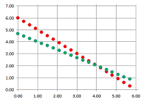
The initial solution has the following geometric meaning. We can think of the two equations $$\begin{array}{ll} x&+y &= 6 ,\\ 2x&+3y &= 14, \end{array}$$ as representations of two lines on the plane. Then the solution $(x,y)=(4,2)$ is the point of their intersection:

The new point of view is very different: instead of the locations, we are after the directions.

We are to solve a vector equation; i.e., to find these unknown coefficients: $$x\cdot\left[\begin{array}{c}1\\2\end{array}\right]+y\cdot\left[\begin{array}{c}1\\3\end{array}\right]=\left[\begin{array}{c}6\\14\end{array}\right].$$ In other words, we need to find a way to stretch these two vectors so that the resulting combination is the vector on the right:

Matrix multiplication

Vectors are matrices: columns and rows. What is the meaning of the dot product then?

Consider: $$\left[ \begin{array}{} 1 & 2 & 0 & 1 & -1 \end{array} \right] \left[ \begin{array}{} 1 \\ 0 \\ 2 \\ 3 \\ 2 \end{array} \right] = \left[ \begin{array}{} 2 \end{array} \right]$$

Idea: Match a row of $A$ and a column of $B$, pairwise multiply, then add the results. The sum is a single entry in $AB$!

In the simplest case above, we have a $1 \times 5$ multiplied with a $5 \times 1$. We think of the $5$'s as cancelling to yield a $1 \times 1$ matrix.

Let's see where $2$ comes from. Here's the algebra: $$\begin{array}{} & 1 & 2 & 0 & 1 & -1 \\ \times & 1 & 0 & 2 & 3 & 2 \\ \hline \\ & 1 +& 0 +& 0 +& 3 -& 2 =2 \end{array}$$ We multiply vertically then add the results horizontally.

Note: the product of a $1 \times 5$ matrix and a $5 \times 1$ matrix.

Example. Even though these are the same two matrices, this is on the opposite end of the spectrum (the columns and rows are very short):

$$\left[ \begin{array}{} 1 \\ 0 \\ 2 \\ 3 \\ 2 \end{array} \right] \left[ \begin{array}{} 1 & 2 & 0 & 1 & -1 \end{array} \right] = \left[ \begin{array}{} 1 & 2 & 0 & 1 & -1 \\ 0 & 0 & 0 & 0 & 1 \\ 2 & 4 & 0 & 2 & -2 \\ \vdots \end{array} \right]$$ Here the left hand side is $5 \times 1$ multiplied with a $1 \times 5$ yielding a $5 \times 5$. It's very much like the multiplication table. $\square$

Example. $$\left[ \begin{array}{} 1 & 2 & 0 \\ 3 & 4 & 1 \end{array} \right] \left[ \begin{array}{} 1 & 2 \\ 0 & 1 \\ 1 & 1 \end{array} \right] = \left[ \begin{array}{} 1\cdot 1 + 2 \cdot 0 + 0\cdot 1 & ... \\ \vdots \end{array} \right]$$ Here we have a $2 \times 3$ multiplied with a $3 \times 2$ to yield a $2 \times 2$. $\square$

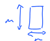
So, an $m \times n$ matrix is a table of real numbers with $m$ rows and $n$ columns:

.

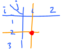
Notation: $A = \{a_{ij}\}$ (or $[a_{ij}]$). Here $a_{ij}$ represents the position in the matrix:

Where is $a_{2,1}$? It's the entry at the $2^{\rm nd}$ row, $1^{\rm st}$ column: $$a_{21}=3\ \longleftrightarrow\ A = \left[ \begin{array}{} (*) & (*) \\ 3 & (*) \\ (*) & (*) \end{array} \right]$$

One can also think of $a_{ij}$ as a function of two variables, when the entries are give by a formula.

Example. $A = \{i+j\}$, $3 \times 3$, what is it? $$a_{ij} = i+j.$$ To find the entries plug in $i=1,2,3$ and $j=1,2,3$: $$\begin{array}{} a_{11} &= 1 + 1 &= 2 \\ a_{12} &= 1+2 &= 3 \\ a_{13} &= 1+3 &= 4 \\ {\rm etc} \end{array}$$ Now form a matrix: $$\left[ \begin{array}{c|ccc} i \setminus j & 1 & 2 & 3 \\ \hline \\ 1 & 2 & 3 & 4 \\ 2 & 3 & 4 & 5 \\ 3 & 4 & 5 & 6 \end{array} \right]$$ What's the difference from a function? Compare $a_{ij}$ with $f(x,y)=x+y$. First, $i,j$ are positive integers, while $x,y$ are real. Second the function is defined on the $(x,y)$-plane:

For the matrix it looks the same, but, in fact, it's “transposed” and flipped, just as in a spreadsheet: $$\begin{array}{lll} &1&2&3&...&n\\ 1\\ 2\\ ...\\ m \end{array}$$

Algebra of matrices...

Let's concentrate on a single entry in the product $C=\{c_{pq}\}$ of matrices $A=\{a_{ij}\},B=\{b_{ij}\}$. Observe, $c_{pq}$ is the "inner product" of $p^{\rm th}$ row of $A$ and $q^{\rm th}$ column of $B$. Consider:

• $p$th row of $A$ is (first index $p$)

$\left[ \begin{array}{} a_{p1} & a_{p2} & ... & a_{pn} \end{array} \right]$

• $q^{\rm th}$ column of $B$ is (second index, $q$)

$$\left[ \begin{array}{} b_{1q} \\ b_{2q} \\ \vdots \\ b_{nq} \end{array} \right]$$ So, $$c_{pq} = a_{p1}b_{1q} + a_{p2}b_{2q} + ...+ a_{pn}b_{nq}.$$ Now we can write the whole thing, the matrix product of an $n \times m$ matrix $\{a_{ij}\}$ and an $m \times k$ matrix $\{b_{ij}\}$ is $C = \{c_{pq}\}$, an $n \times k$ matrix with $$c_{pq} = \sum_{i=1}^n a_{pi}b_{iq}.$$

When can we both add and multiply? Given $m \times n$ matrix $A$ and $p \times q$ matrix $B$,

• 1. $A+B$ makes sense only if $m=p$ and $n=q$.
• 2. $AB$ makes sense only if $n=p$.

Both make sense only if both $A,B$ are $n \times n$. These are called square matrices.

Linear functions are matrices and matrices are linear functions

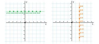
Linear functions on the plane..

Example (collapse on axis). The latter is the “degenerate” case such as the following. Let's consider this very simple function: $$\begin{cases}u&=2x,\\ v&=0,\end{cases} \ \leadsto\ \left[ \begin{array}{} u \\ v \end{array}\right]= \left[\begin{array}{} 2 & 0 \\ 0 & 0 \end{array} \right] \cdot \left[ \begin{array}{} x \\ y \end{array} \right]$$ Below, one can see how this function collapses the whole plane to the $x$-axis:

In the mean time, the $x$-axis is stretched by a factor of $2$. $\square$

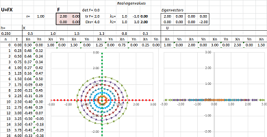
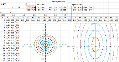
Example (stretch-shrink along axes). Let's consider this function: $$\begin{cases}u&=2x,\\ v&=4y.\end{cases}$$ Here, this linear function is given by the matrix: $$F=\left[ \begin{array}{ll}2&0\\0&4\end{array}\right].$$

What happens to the rest of the plane? Since the stretching is non-uniform, the vectors turn. However, this is not a rotation but rather “fanning out”:

$\square$

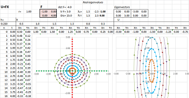
Example (stretch-shrink along axes). A slightly different function is: $$\begin{cases}u&=-x,\\ v&=4y.\end{cases} $$ It is simple because the two variables are fully separated.

The slight change to the function produces a similar but different pattern: we see the reversal of the direction of the ellipse around the origin. Here, the matrix of $F$ is diagonal: $$F=\left[ \begin{array}{ll}-1&0\\0&4\end{array}\right].$$ $\square$

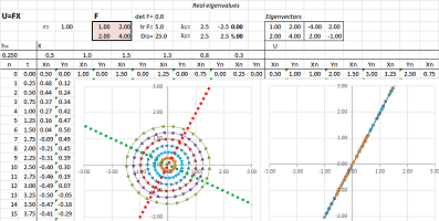
Example (collapse). Let's consider a more general linear function: $$\begin{cases}u&=x&+2y,\\ v&=2x&+4y,\end{cases} \ \Longrightarrow\ F=\left[ \begin{array}{cc}1&2\\2&4\end{array}\right].$$

It appears that the function has a stretching in one direction and a collapse in another.

The determinant is zero: $$\det F=\det\left[ \begin{array}{cc}1&2\\2&4\end{array}\right]=1\cdot 4-2\cdot 2=0.$$ That's why there is a whole line of points $X$ with $FX=0$. To find it, we solve this equation: $$\begin{cases}x&+2y&=0,\\ 2x&+4y&=0,\end{cases} \ \Longrightarrow\ x=-2y.$$ $\square$

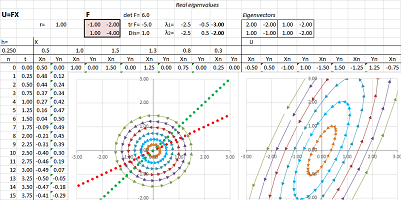
Example (stretch-shrink). Let's consider this function: $$\begin{cases}u&=-x&-2y,\\ v&=x&-4y.\end{cases} $$ Here, the matrix of $F$ is not diagonal: $$F=\left[ \begin{array}{cc}-1&-2\\1&-4\end{array}\right].$$

$\square$

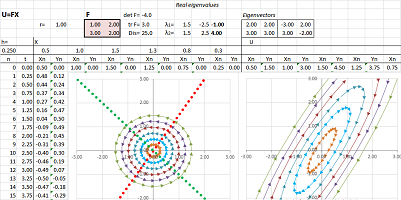
Example (stretch-shrink). Let's consider this linear function: $$\begin{cases}u&=x&+2y,\\ v&=3x&+2y.\end{cases} $$ Here, the matrix of $F$ is not diagonal: $$F=\left[ \begin{array}{cc}1&2\\3&2\end{array}\right].$$

$\square$

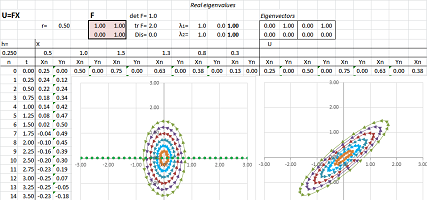
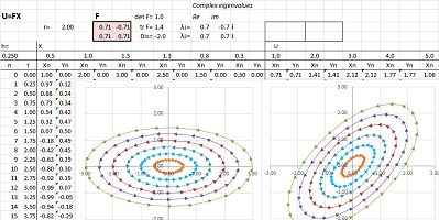
Example (skewing-shearing). Consider a matrix with repeated (and, therefore, real) eigenvalues: $$F=\left[ \begin{array}{cc}-1&2\\0&-1\end{array}\right].$$ Below, we replace a circle with an ellipse to see what happens to it under such a function:

There is still angular stretch-shrink but this time it is between the two ends of the same line. To see clearer, consider what happens to a square:

The plane is skewed, like a deck of cards:

Another example is when wind blows at the walls with its main force at their top pushing in the direction of the wind while their bottom is held by the foundation. Such a skewing can be carried out with any image editing software such as MS Paint. $\square$

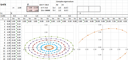
Example (rotation). Consider a rotation through $90%$ degrees: $$\begin{cases}u&=& -y,\\ v&=x&&,\end{cases} \ \leadsto\ \left[ \begin{array}{} u \\ v \end{array}\right] = \left[\begin{array}{} 0&1\\-1&0 \end{array} \right] \cdot \left[ \begin{array}{} x \\ y \end{array} \right]$$

Consider a rotation through $45%$ degrees: $$\begin{cases}u&=\cos \pi/4\ x& -\sin \pi/4\ y,\\ v&=\sin \pi/4\ x&+\cos \pi/4\ y&.\end{cases} \ \leadsto\ \left[ \begin{array}{} u \\ v \end{array}\right] = \left[\begin{array}{rrr} \cos \pi/4\ y & -\sin \pi/4\ y \\ \sin \pi/4\ y & \cos \pi/4\ y \end{array} \right] \cdot \left[ \begin{array}{} x \\ y \end{array} \right]$$

$\square$

Example (rotation with stretch-shrink). Let's consider a more complex function: $$\begin{cases}u&=3x&-13y,\\ v&=5x&+y.\end{cases} $$ Here, the matrix of $F$ is not diagonal: $$F=\left[ \begin{array}{cc}3&-13\\5&1\end{array}\right].$$

$\square$

Matrix operations

The properties of matrix multiplication are very much like the ones for numbers.

What's not working is commutativity: $$AB \neq BA,$$ generally. Indeed, let try to put random numbers in two matrices and see if they “commute”: $$\begin{array}{lll} \left[\begin{array}{lll} 1&2\\ 2&3 \end{array}\right] \cdot \left[\begin{array}{lll} 2&1\\ 2&3 \end{array}\right] = \left[\begin{array}{lll} 2\cdot 2+2\cdot 2=6&\square\\ \square&\square \end{array}\right] &\text{ Now in reverse...} \\ \left[\begin{array}{lll} 2&1\\ 2&3 \end{array}\right] \cdot \left[\begin{array}{lll} 1&2\\ 2&3 \end{array}\right] = \left[\begin{array}{lll} 2\cdot 1+1\cdot 2=4&\square\\ \square&\square \end{array}\right] &\text{ ...already different!} \end{array}$$

To understand the idea of non-commutativity one might think about matrices as operation carried out in manufacturing. Suppose $A$ is polishing and $B$ is painting. Clearly, $$AB \neq BA.$$

Mathematically, we have: $$\begin{array}{} x \stackrel{A}{\rightarrow} y \stackrel{B}{\rightarrow} z\\ x \stackrel{B}{\rightarrow} y \stackrel{A}{\rightarrow} z \end{array}$$ Does the results have to be the same? Not in general. Let's put them together: $$ \newcommand{\ra}[1]{\!\!\!\!\!\!\!\xrightarrow{\quad#1\quad}\!\!\!\!\!} \newcommand{\da}[1]{\left\downarrow{\scriptstyle#1}\vphantom{\displaystyle\int_0^1}\right.} % \begin{array}{llllllllllll} x & \ra{A} & y \\ \da{B} & \searrow ^C & \da{B} \\ y & \ra{A} & z \end{array} $$ This is called a commutative diagram if $C$ makes sense, i.e., $C=AB=BA$.

Let's, again, think of matrices as functions. Then non-commutativity isn't surprising. Indeed, take $$f(x)=\sin x,\ g(x)=e^x.$$ Then $$\begin{array}{} gf &\neq fg ;\\ e^{\sin x} &\neq \sin e^x \end{array}$$ Functions don't commute, in general, and neither do matrices.

But some do commmute. For example, $A^2=A \cdot A$ makes sense, as well as: $$A^n = A \cdot ... \cdot A$$ (where there are $n$ $A$'s). Then $$A^m \cdot A^n = A^n A^m,$$ i.e., powers commute.

Also, consider diagonal matrices $A = \{a_{ij}\}$ with $a_{ij}=0$ if $i \neq j$. Such a matrix commute with any matrix. In particular, define $$I_n = \left[ \begin{array}{} 1 & 0 & 0 & ... \\ 0 & 1 & 0 & ... \\ \vdots \\ 0 & 0 & ... & 1 \end{array} \right]$$ or, $$a_{ij}=\left\{ \begin{array}{} 1 & i = j \\ 0 & {\rm otherwise}. \end{array} \right.$$ It is called the identity matrix.

Proposition. $IA=A$ and $AI=A$.

Provided, of course, $A$ has the appropriate dimensions:

• $I_nA=A$ makes sense if $A$ is $n \times m$.
• $AI_n=A$ makes sense if $A$ is $m \times n$.

Proof. Go back to the definition: for $AI_n=A$. Suppose $AI_n = \{c_{pq}\}$: $$c_{pq} = a_{p1}b_{1q} + a_{p2}b_{2q} + ... + a_{pn}b_{nq}. (AB)$$ But $$b_{iq} = \left\{ \begin{array}{} 1 & i=q \\ 0 & i \neq q \end{array} \right. ,$$ so $$b_{iq}=0,0,...,0,1,0,...,0.$$ Substitute these: $$c_{pq}=a_{p1}\cdot 0 + a_{p2} \cdot 0 + ... + a_{p,q-1}\cdot 0 + a_{pq}\cdot 1 + a_{p,q+1} \cdot 0 + ... + a_{pn} \cdot 0 = a_{pq}.$$ The left hand side is the $pq$ entry of $AI_n$ and the right hand side is the $pq$ entry of $A$, so $AI_n = A$. The proof of the other identity $I_nA=A$ is similar. $\blacksquare$

So, $I_n$ behaves like $1$ among numbers.

Both addition and multiplication can be carried out for $n \times m$ matrices, $n$ fixed.

You can take this idea quite far. We can define the exponent of a matrix $A$: $$e^A=I + A + \frac{1}{2}A^2 + \frac{1}{3!}A^3 + ... + \frac{1}{n!}A^n + ... $$

Theorem (Properties of matrix multiplication).

• Associative Law 1: $(AB)C=A(BC)$.
• Associative Law 2: $r(AB)=A(rB)=(rA)B$.
• Distributive Law 1: $A(B+C)=AB+AC$.
• Distributive Law 2: $(B+C)A = BA + CA$.

Proof. Suppose $$A = \{a_{ij}\},\ B=\{b_{ij}\},\ C=\{c_{ij}\},$$ and $$B+C=D=\{d_{ij}\},\ S=(B+C)A = \{s_{ij}\}.$$ Consider: $$s_{pq} = d_{p1}a_{1q} + d_{p2}a_{2q} + ... + d_{pn}a_{nq},$$ where $d_{ij}=b_{ij}+c_{ij}$. Substitute $$s_{pq} = (b_{p1}+c_{p1})a_{1q} + (b_{p2}+c_{p2})q_{2q} + ... + (b_{pn}+c_{pn})a_{nq}$$ expand and rearrange $$\begin{array}{} &= b_{p1}a_{1q} + c_{p1}a_{1q} + ... + b_{pn}a_{nq} + c_{pn}a_{nq} \\ &= (b_{p1}a_{1q}+...+b_{pn}a_{nq}) + (c_{p1}a_{1q} + ... + c_{pn}a_{nq}) \\ &= pq \text{ entry of } BA + pq \text{ entry of } CA. \end{array}$$ So $(B+C)A = BA + CA$. $\blacksquare$

Let's rewrite this computation with $\Sigma$-notation. $$\begin{array}{} s_{pq} &= \sum_{i=1}^n d_{pi}a_{iq} \\ &= \sum_{i=1}^n(b_{pi}+c_{pi})a_{iq} \\ &= \sum_{i=1}^n(b_{pi}a_{iq} + c_{pi}a_{iq}) \\ &= \sum_{i=1}^nb_{pi}a_{iq} + \sum_{i=1}^n c_{pi}a_{iq}. \end{array}$$

Back to systems of linear equations. Recall

• equation: $ax=b$, $a \neq 0 \rightarrow$ solve $x=\frac{b}{a}$
• system: $AX=B$, ?? $\rightarrow$ solve $X = \frac{B}{A}$.

To do that we need to define division of matrices!

Specifically, define an analogue of the reciprocal $\frac{1}{a}$, the inverse $A^{-1}$. Both notation and meaning are of the inverse function!

But is it $X=BA^{-1}$ or $A^{-1}B$? We know these don't have to be the same! We define division via multiplication. Recall:

• $x=\frac{1}{a}$ if $ax=1$ or $xa=1$.

Similarly,

• $X=A^{-1}$ if $AX=I$ or $XA=I$.

Question: Which one is it? Answer: Both!

The first one is called the "right-inverse" of $A$ and the second one is called the "left-inverse" of $A$.

Definition. Given an $n \times n$ matrix $A$, its inverse is a matrix $B$ that satisfies $AB=I$, $BA=I$.

Note: "its" is used to hide the issue. It should be "an inverse" or "the inverse".

Question: Is it well defined? Existence: not always.

How do we know? As simple as this. Go to $n=1$, then matrices are numbers. Then $A=0$ does not have the inverse.

Definition. If the inverse exists, $A$ is called invertible. Otherwise, $A$ is singular.

Theorem. If $A$ is invertible, then its inverse is unique.

Proof. Suppose $B,B'$ are inverses of $A$. Then (compact proof): $$B=BI=B(AB')=(BA)B'=IB'=B'.$$ With more details, try (1) $BA=I$ and (2) $AB'=I$. Multiply the equation by $B'$ on both sides: $$(BA)B'=IB'.$$ Use associativity on the left and the definition of multiplicative inverse on the right: $$B(AB')=B'.$$ Use the second equation: $$BI=B'.$$ Use the definition of multiplicative inverse on the left: $$B=B'.$$ $\blacksquare$

So, if $A$ is invertible, then $A^{-1}$ is the inverse.

Example. What about $I$? $I^{-1}=I$, because $II=I$. $\square$

Example. Verify: $$\left[ \begin{array}{} 3 & 0 \\ 0 & 3 \end{array} \right]^{-1} = \left[ \begin{array}{} \frac{1}{3} & 0 \\ 0 & \frac{1}{3} \end{array} \right]$$ It can be easily justified without computation: $$(3I)^{-1} = \frac{1}{3}I.$$

Generally, given $$A = \left[ \begin{array}{} a & b \\ c & d \end{array} \right],$$ find the inverse.

Start with: $$A^{-1} = \left[ \begin{array}{} x & y \\ u & v \end{array} \right].$$ Then $$\left[ \begin{array}{} a & b \\ c & d \end{array} \right] \left[ \begin{array}{} x & y \\ u & v \end{array} \right] = \left[ \begin{array}{} 1 & 0 \\ 0 & 1 \end{array} \right]$$ Solve this matrix equation. Expand: $$\left[ \begin{array}{} ax+ba & ay+bv \\ cx+du & cy+dv \end{array} \right] = \left[ \begin{array}{} 1 & 0 \\ 0 & 1 \end{array} \right]$$ Break apart: $$\begin{array}{} ax+bu=1, & ay+bv=0 \\ cx+du=0, & cy+dv=1 \end{array}$$ The equations are linear.

Exercise. Solve the system.

A shortcut formula: $$A^{-1}=\frac{1}{ad-bc} \left[ \begin{array}{} d & -b \\ -c & a \end{array} \right]$$

Let's verify: $$\begin{array}{} AA^{-1} &= \left[ \begin{array}{} a & b \\ c & d \end{array} \right] \frac{1}{ad-bc} \left[ \begin{array}{} d & -b \\ -c & a \end{array} \right] \\ &= \frac{1}{ad-bc}\left[ \begin{array}{} a & b \\ c & d \end{array} \right] \left[ \begin{array}{} d & -b \\ -c & a \end{array} \right] \\ &= \frac{1}{ad-bc} \left[ \begin{array}{} ad-bc & ab-ba \\ cd - dc & -bc + da \end{array} \right] \\ &= \left[ \begin{array}{} 1 & 0 \\ 0 & 1 \end{array} \right] = I \end{array}$$ $\square$

Exercise. Verify also $A^{-1}A=I$.

To find $A^{-1}$, solve a system. And it might not have a solution: $\frac{1}{ad-bc} = ?$.

Fact: For $$A=\left[ \begin{array}{} a & b \\ c & d \end{array} \right],$$ the inverse $A^{-1}$ exists if and only if $ad-bc \neq 0$. Here, $D=ad-bc$ is called the determinant of $A$.

Example. $$0 = \left[ \begin{array}{} 0 & 0 \\ 0 & 0 \end{array} \right]$$ is singular, by formula. $\square$

In dimension $n$, the zero matrix is singular: $0 \cdot B = 0$, not $I$. Then, just like with real numbers, $\frac{1}{0}$ undefined.

Example. Other singular matrices: $$\left[ \begin{array}{} 1 & 1 \\ 1 & 1 \end{array} \right], \left[ \begin{array}{} 0 & 0 \\ 0 & 1 \end{array} \right], \left[ \begin{array}{} 1 & 3 \\ 1 & 3 \end{array} \right]$$

What do they have in common?

What if we look at them as pairs of vectors: $$\left\{ \left[ \begin{array}{} 1 \\ 1 \end{array} \right], \left[ \begin{array}{} 1 \\ 1 \end{array} \right] \right\}, \left\{ \left[ \begin{array}{} 0 \\ 0 \end{array} \right], \left[ \begin{array}{} 0 \\ 1 \end{array} \right] \right\}, \left\{ \left[ \begin{array}{} 1 \\ 1 \end{array} \right], \left[ \begin{array}{} 3 \\ 3 \end{array} \right] \right\}$$

What's so special about them as opposed to this: $$\left\{ \left[ \begin{array}{} 1 \\ 0 \end{array} \right], \left[ \begin{array}{} 0 \\ 1 \end{array} \right] \right\}$$ The vector are linearly dependent! $\square$

Theorem. If $A$ is invertible, then so is $A^{-1}$. And $({A^{-1}})^{-1}=A$.

Proof. $\blacksquare$

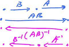
Theorem. If $A,B$ are invertible, then so is $AB$, and $$(AB)^{-1} = B^{-1}A^{-1}.$$

This can be explained by thinking about matrices as functions:

Proof. $\blacksquare$

Determinants

Given a matrix or a linear operator $A$, it is either singular or non-singular: $${\rm ker \hspace{3pt}}A \neq 0 {\rm \hspace{3pt} or \hspace{3pt}} {\rm ker \hspace{3pt}}A=0$$

If the kernel is zero, then $A$ is invertible. Recall, matrix $A$ is singular when its column vectors are linearly dependent ($i^{\rm th}$ column of $A = A(e_i)$).

The goal is to find a function that determines whether $A$ is singular. It is called the determinant.

Specifically, we want: $${\rm det \hspace{3pt}}A = 0 {\rm \hspace{3pt} iff \hspace{3pt}} A {\rm \hspace{3pt} is \hspace{3pt} singular}.$$

Start with dimension $2$. $A = \left[ \begin{array}{} a & b \\ c & d \end{array} \right]$ is singular when $\left[ \begin{array}{} a \\ c \end{array} \right]$ is a multiple of $\left[ \begin{array}{} b \\ d \end{array} \right]$

Let's consider that: $$\left[ \begin{array}{} a \\ c \end{array} \right] = x\left[ \begin{array}{} b \\ d \end{array} \right] \rightarrow \begin{array}{} a = bx \\ c = dx \\ \end{array}$$ So $x$ has to exist. Then, $$x=\frac {a}{b} = \frac{c}{d}.$$ That the condition. (Is there a division by 0 here?)

Rewrite as: $ad-bc=0 \longleftrightarrow A$ is singular, and we want $\det A =0$.This suggests that $${\rm det \hspace{3pt}}A = ad-bc,$$

Let's make this the definition.

Theorem. A $2\times 2$ matrix $A$ is singular iff $\det A=0$.

Proof. ($\Rightarrow$) Suppose $\left[ \begin{array}{} a & b \\ c & d \end{array} \right]$ is singular, then $\left[ \begin{array}{} a \\ c \end{array} \right] = x \left[ \begin{array}{} b \\ d \end{array} \right]$, then $a=xb, c=xd$, then substitute:

$${\rm det \hspace{3pt}}A = ad-bc = (xb)d - b (xd)=0.$$

($\Leftarrow$) Suppose $ad-bc=0$, then let's find $x$, the multiple.

• Case 1: assume $b \neq 0$, then choose $x = \frac{a}{b}$. Then

$$\begin{array}{} xb &= \frac{a}{b}b &= a \\ xd &= \frac{a}{b}d &= \frac{ad}{b} = \frac{bc}{b} = c. \end{array}$$ So $$x \left[ \begin{array}{} b \\ d \end{array} \right] = \left[ \begin{array}{} a \\ c \end{array} \right].$$

• Case 2: assume $a \neq 0$, etc.

We defined $ \det A$ with requirement that $ \det A = 0$ iff $A$ is singular.

But $ \det A$ could be $k(ad-bc)$, $k \neq 0$. Why $ad-bc$?

Because...

• Observation 1: $ \det I_2=1$

• Observation 2: Each entry of $A$ appears only once.

What if we interchange rows or columns? $$ \det \left[ \begin{array}{} c & d \\ a & b \end{array} \right] = cb-ad = - \det \left[ \begin{array}{} a & b \\ c & d \end{array} \right].$$ Then the sign changes. So

• Observation 3: $ \det A=0$ is preserved under this elementary row operation.

Moreover, $ \det A$ is preserved up to a sign! (later)

• Observation 4: If $A$ has a zero row or column, then $ \det A=0$.

To be expected -- we are talking about linear independence!

• Observation 5: $ \det A^T= \det A$.

$$ \det \left[ \begin{array}{} a & c \\ b & d \end{array} \right] = ad-bc$$

• Observation 6: Signs of the terms alternate: $+ad-bc$.
• Observation 7: $ \det A \colon {\bf M}(2,2) \rightarrow {\bf R}$ is linear... NOT!

$$\begin{array}{} \det 3\left[ \begin{array}{} a & b \\ c & d \end{array} \right] &= \det \left[ \begin{array}{} 3a & 3b \\ 3c & 3d \end{array} \right] \\ &= 3a3d-3b3c \\ &= 9(ad-bc) \\ &= 9 \det \left[ \begin{array}{} a & b \\ c & d \end{array} \right] \end{array}$$ not linear, but quadratic. Well, not everything in linear algebra has to be linear...

Let's try to step up from dimension 2 with this simple matrix:

$$B = \left[ \begin{array}{} e & 0 & 0 \\ 0 & a & b \\ 0 & c & d \end{array} \right]$$

We, again, want to define ${\rm det \hspace{3pt}}B$ so that ${\rm det \hspace{3pt}}B=0$ if and only if $B$ is singular, i.e., the columns are linearly dependent.

Question: What does the value of $e$ do to the linear dependence?

• Case 1, $e=0 \rightarrow B$ is singular. So, $e=0 \rightarrow {\bf det \hspace{3pt}}B=0$.
• Case 2, $e \neq 0 \rightarrow$ the vectors are:

$$\left[ \begin{array}{} e & 0 & 0 \\ 0 & a & b \\ 0 & c & d \end{array} \right]$$ and $v_1=\left[ \begin{array}{} e \\ 0 \\ 0 \end{array} \right]$ is not a linear combination of the other two $v_2,v_3$.

So, we only need to consider the linear independence of those two, $v_2,v_3$!

Observe that $v_2,v_3$ are linearly independent if and only if ${\rm det \hspace{3pt}}A \neq 0$, where $$A = \left[ \begin{array}{} a & b \\ c & d \end{array} \right]$$

Two cases together: $e=0$ or ${\rm det \hspace{3pt}}A=0 \longleftrightarrow B$ is singular.

So it makes sense to define: $${\rm det \hspace{3pt}}B = e \cdot {\rm det \hspace{3pt}}A$$ With that we have: ${\rm det \hspace{3pt}}B=0$ if and only if $B$ is singular.

Let's review the observations above...

• (1) $\det I_3 = 1$.
• (4), (5) still hold.
• (7) still not linear: $\det (2B) = 8 \det B.$

It's cubic.

So far so good...

Now let's give the definition of ${\rm det}$ in dimension three.

Definition in dimension 3 via that in dimension 2...

We define via "expansion along the first row."

$A = $

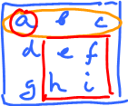
$$\det A = a \det \left[ \begin{array}{} e & f \\ h & i \end{array} \right] - b \det \left[ \begin{array}{} d & f \\ g & i \end{array} \right] + c \det \left[ \begin{array}{} d & e \\ g & h \end{array} \right]$$ Observe that the first term is familiar from before.

Expand farther using the formula for $2 \times 2$ determinant: $$\begin{array}{} {\det} _1 A &= a(ei-fh) - b(di-fg)+c(dh-eg) \\ &= (aei+bfg+cdh)-(afh+bdi+ceg) \end{array}$$

Observe:

• each entry appears twice -- once with $+$, once with $-$.

Prior observation:

• in each term (in determinant) every column appears exactly once, as does every row.

The determinant helps us with problems from before.

Example. Given $(1,2,0),(-1,0,2),(2,-2,1)$. Are they linearly independent? We need just yes or no; no need to find the actual dependence.

Note: this is similar to discriminant that tells us how many solutions a quadratic equation has:

• $D<0 \rightarrow 0$ solutions,
• $D=0 \rightarrow 1$ solution,
• $D>0 \rightarrow 2$ solutions.

Consider: $$\begin{array}{} \det \left[ \begin{array}{} 1 & -1 & 2 \\ 2 & 0 & -2 \\ 3 & 2 & 1 \end{array} \right] &= 1 \cdot 0 \cdot 1 + (-1)(-2)3 + 2\cdot 2 \cdot 2 - 3 \cdot 0 \cdot 2 - 1(-2)2 - 2(-1)1 \\ &= 6 + 8 + 4 + 2 \\ &\neq 0 \end{array}$$ So, they are linearly independent.

Back to matrices.

Recall the definition, for:

$A = \left[ \begin{array}{} a & b & c \\ d & e & f \\ g & h & i \end{array} \right]$ of expansion along the first row:

(*) $$\begin{array}{} {\det} _1A &= a \det \left[ \begin{array}{} e & f \\ h & i \end{array} \right] - b \det \left[ \begin{array}{} d & f \\ g & i \end{array} \right]+ c \det \left[ \begin{array}{} d & e \\ g & h \end{array} \right] \\ &=(aei+bfg+cdh)-(afh+bdi+ceg) \end{array}$$ Let's try the expansion along the second row.

(**) $$\begin{array}{} {\det} _2A &= d \det \left[ \begin{array}{} b & c \\ h & i \end{array} \right] - e \det \left[ \begin{array}{} a & c \\ g & i \end{array} \right] + f \det \left[ \begin{array}{} a & b \\ g & h \end{array} \right] \\ &=d(bi-ha) - e(ai-cg) + f(ah-bg) \\ &=dbi+\ldots \end{array}$$ Let' try to match $(*)$ and $(**)$.

Wrong sign! But it's wrong for all terms, fortunately!

To fix the formula, flip the signs, $$\begin{array}{} {\det}_{2} A &= -d \det \left[ \begin{array}{} b & c \\ h & i \end{array} \right] + e \det \left[ \begin{array}{} a & c \\ g & i \end{array} \right] - f \det \left[ \begin{array}{} a & b \\ g & h \end{array} \right] \end{array}$$

Conclusion: the expansion formula depends on the row chosen.

But it's the same procedure:

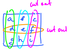
• $3$ determinants, $2 \times 2$,
• with coefficients cut out row and column,
• signs alternate.

The difference is alternating signs: start with $-$ or $+$, depending on the row chosen.

The derivative is a matrix

The partial derivatives of a function of several variables form a vector, in dimension $2$: $$\begin{array}{cccccccccccc} &&&& &f\\ &&&&\swarrow_x&&_y\searrow\\ &&\nabla f=<&f_x& && &f_y&>\\ \end{array}$$ and in dimension $3$: $$\begin{array}{cccccccccccc} &&&& &&&f\\ &&&&\swarrow_x&&&\downarrow_y&&&_z\searrow\\ &&\nabla f=<&f_x& && &f_y& && &f_z&>\\ \end{array}$$ In the mean time, the second partial derivatives of a function of several variables form a matrix, in dimension $2$: $$\begin{array}{cccccccccccc} &&&& &f\\ &&&&\swarrow_x&&_y\searrow\\ &&&f_x& && &f_y\\ &&\swarrow_x&&_y\searrow&&\swarrow_x&&_y\searrow\\ &f_{xx}&&&&f_{yx}\quad f_{xy}&&&&f_{yy}\\ \end{array}$$

Definition. Suppose that $z=f(x,y)$ is a differentiable function of two variables. The Hessian $H$ of $f$ is the $2\times 2$ matrix of second partial derivatives of $f$: $$H = \left[ \begin{array}{lll}f_{xx} &f_{xy}\\f_{yx} &f_{yy} \end{array} \right].$$

But the second derivative is just the derivative of the derivative!

And in dimension $3$: $$\begin{array}{cccccccccccc} &&&& &&&f\\ &&&&\swarrow_x&&&\downarrow_y&&&_z\searrow\\ &&&f_x& && &f_y& && &f_z\\ &&\swarrow_x&\downarrow_y&_z\searrow&&\swarrow_x&\downarrow_y&_z\searrow&&\swarrow_x&\downarrow_y&_z\searrow\\ &f_{xx}&&f_{yx}&&f_{zx}\quad f_{xy}&&f_{yy}&&f_{zy}\quad f_{xz}&&f_{xz}&&f_{yz}\ f_{zz}\\ \end{array}$$

Definition. Suppose that $u=f(x,y,z)$ is a differentiable function of three variables. The Hessian $H$ of $f$ is the $3\times 3$ matrix of second partial derivatives of $f$: $$H = \left[ \begin{array}{lll} f_{xx} &f_{xy}&f_{xz}\\ f_{yx} &f_{yy}&f_{yz}\\ f_{zx} &f_{zy}&f_{zz} \end{array} \right].$$

According to Clauraut's theorem, the matrix is symmetric. This is a matrix of four functions of two variables or, better, a matrix-valued function of two variables.

Define $$D=\det H = f_{xx}f_{yy} - f_{xy}^2.$$

Theorem (Second Derivative Test dimension $2$). Suppose $(a,b)$ is a critical point of $z=f(x)$. Then

• if $D(a,b)>0$ and $f_{xx}(a,b)>0$ then $(a,b)$ is a local minimum of $f$.
• if $D(a,b)>0$ and $f_{xx}(a,b)<0$ then $(a,b)$ is a local maximum of $f$.
• if $D(a,b)<0$ then $(a,b)$ is a saddle point of $f$.

When $D(a,b)=0$, the second derivative test is inconclusive: the point could be any of a minimum, maximum or saddle point.

Flow integrals on the plane

Let's review the recent integral that involved parametric curves.

Suppose $X=X(t)$ is a parametric curve on $[a,b]$. The first is the (component-wise) integral of the parametric curve: $$\int_a^bX(t)\, dt,$$ providing the displacement from the known velocity, as functions of time. The second is the arc-length integral: $$\int_C f\, dx=\int_a^bf(X(t))||X'(t)||\, dt,$$ providing the mass of a curve of variable density. The third is the line integral along an oriented curve: $$\int_C F\, dX=\int_a^bF(X(t))\cdot X'(t)\, dt,$$ providing the work of the force field. There is one more, the line integral across an oriented curve: $$\int_C F\, dX^\perp=\int_a^bF(X(t))\cdot X'(t)^\perp\, dt,$$ providing the flux of the velocity field (it is explained in this section). The main difference between the first and the rest is that the parametric curve isn't the integrand (and the output is another parametric curve) but a way to set up the domain of integration (and the output is a number).

The analysis appears to mimic that of line integrals (work). The setup is exactly the same: a vector field and a curve.

But this time the nature of the two is very different: force vs. velocity and path vs. front. We then are not after the tangent components of the vector field but after its normal components:

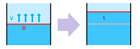
Suppose the flow with a constant speed $V$ has the front of width $D$.

Then the flux $W$ is equal to their product of these two numbers: $$L=V\cdot D.$$ The velocity may vary along this edge.

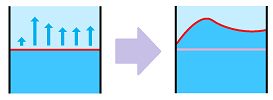
Then, as we have seen, the flux is the integral of this function: $$L=\int_D V(x)\, dx.$$

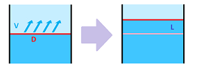
We now proceed (and will limit ourselves) to the $2$-dimensional case. We start with a constant velocity and a linear front... They may be misaligned as in the case of a wave hitting the shore:

In addition to motion “in” and “out” (as well as “left-right” and “up-down”), the third possibility emerges: what if the flow is parallel to the chosen front? Then the flux is zero. There are, of course, diagonal directions. Suppose the flow with a constant speed $V$ has the front of width $D$. Then the flux is the area swept by the progressing front:

In order to find and discard the irrelevant part of the velocity $V$, we decompose it into parallel and perpendicular components relative to $D$ just as before: $$V=V_{||}+V_\perp.$$ In contrast to the force, we pick the other component! The relevant part of the velocity $V$ is its “normal” component.

File:Projection of velocity on normal.png

It is its projection on the direction perpendicular to the front vector: $$V_{\perp}=||V||\sin \alpha,$$ where $\alpha$ is the angle between $V$ and $D$.

This component is then multiplied by the width of the front to get the flux: $$L=V_{\perp}||D||=||V||\, ||D||\, \sin \alpha.$$

File:Flux of velocity across edge.png

We would like to express this in terms of the dot product just as in the last section. It is the dot product of $V$ but with what vector? It is $D$ rotated $90$ degree counterclockwise: $$L=||V||\, ||D||\, \cos (\pi-\alpha).$$ Recall that the normal vector of a vector $D=<u,v>$ on the plane is given by $$D^\perp=<u,v>^\perp=<-v,u>.$$

Definition. The flux of a plane flow with velocity vector $V$ across the front vector $D$ is defined to be: $$L=V\cdot D^\perp.$$

The flux is proportional to the magnitude of the velocity and to the magnitude of the vector of representing the front.

The definition of flow applies to a straight front... or to a front made of multiple straight edges:

File:Flux across a front.png

If these segments are given by the edge vectors $D_1,...,D_n$ and the velocity for each is given by the vectors $V_1,...,V_n$, then the flux is defined to be the simple sum of the flux across each: $$L=V_1\cdot D^\perp_1+...+V_n\cdot D^\perp_n.$$

The front above is, just as before, given by path of a parametric curve $X=X(t)$. Then, $$D_i=X(t_{i+1})- X(t_i),\ t=0,2,...,n-1.$$ Once again, it doesn't matter how fast the parametrization goes along its path. It is the front itself -- the locations and the angles relative to the flow -- that matters. This is about an oriented curve. In the mean time, the vectors of the flow come from a vector field, $V=V(X)$. In contrast to the last section, this is a velocity field. If its vectors change incrementally, one may be able to compute the flux by a simple summation, as above.

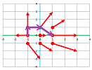
Example. In order to compute the flux of a discrete vector field across a curve made of straight edges $D_1,...,D_n$, all we need is the formula: $$L=\sum_{i=1}^nV_i\cdot D^\perp_i.$$ In order for the computation to make sense, the edges of the front and the vectors of the velocity have to be paired up! Here's a simple example:

We pick the value of the velocity from the initial point of each edge: $$L=<-1,0>\cdot <-1,0>+<0,2>\cdot <0,1>+<1,2>\cdot <-1,1>=4.$$

$\square$

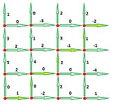
Example. An even simpler situation is when the front is made of the edges of the square grid on the plane. Then there is a velocity vector associated with each edge of the grid, but only one of its components matters: the horizontal when the edge is vertical and the vertical when the edge is horizontal. It is then sufficient to assign a single number to each edge to provide the relevant part of velocity.

Then, for example, the flux across the “staircase” is simply the sum of the values provided: $$L=1+0+0+2+(-1)+1+(-2)=1.$$

$\square$

A vector field that varies continuously from location to location or a curve that continuously changes directions will require approximations.

The general setup for defining and computing flux is identical to what we have done several times. Suppose we have a vector field $V=V(X)$ and an oriented curve $C$. We then find a regular parametrization of the latter: a parametric curve $X=X(t)$ defined on the interval $[a,b]$. We have a sampled partition $P$: $$a=t_0\le c_1\le t_1\le ... \le c_n\le t_n=b.$$ We divide the front into small segments with end-points $X_i=X(t_i)$ and then sample the velocity at the points $C_i=X(c_i)$.

Then the flux across each of these segments is approximated by the flux with the velocity constantly equal to $V(C_i)$: $$\text{ flux across }i\text{th segment}\approx \text{ velocity }\cdot \text{ length}=V(C_i)\cdot D^\perp_i.$$ Then, $$\text{total flux }\approx \sum_{i=1}^n V(X(c_i))\cdot D^\perp_i.$$ This is the formula that we have used and will continue to use for numerical approximations.

Example. Estimate the flux of the velocity field $$V(x,y)=<xy,x-y>$$ across the upper half of the unit circle directed counterclockwise. First we parametrize the curve: $$X(t)=<\cos t,\sin t>,\ 0\le t\le \pi.$$ We choose $n=4$ intervals of equal length with the left-ends as the sample points: $$\begin{array}{lll} x_0=0& x_1=\pi/4& x_2=\pi/2& x_3=3\pi/4&x_4=\pi\\ c_1=0& c_2=\pi/4& c_3=\pi/2& c_4=3\pi/4&\\ X_0=(1,0)& X_1=(\sqrt{2}/2,\sqrt{2}/2)& X_2=(0,1)& X_3=(-\sqrt{2}/2,\sqrt{2}/2)& X_4=(-1,0)\\ & D_1=(\sqrt{2}/2,\sqrt{2}/2)& D_2=(0,1)& D_3=(-\sqrt{2}/2,\sqrt{2}/2)& D_4=(-1,0)\\ & N_1=(\sqrt{2}/2,\sqrt{2}/2)& N_2=(0,1)& N_3=(-\sqrt{2}/2,\sqrt{2}/2)& N_4=(-1,0)\\ C_1=(1,0)& C_2=(\sqrt{2}/2,\sqrt{2}/2)& C_3=(0,1)& C_4=(-\sqrt{2}/2,\sqrt{2}/2)\\ V(C_1)=<0,1>& V(C_2)=<1/2,0>& V(C_3)=<0,-1>& V(C_4)=<-1/2,-\sqrt{2}> \end{array}$$ Then,... $$\begin{array}{lll} W&\approx <0,1>\cdot <\sqrt{2}/2-1,\sqrt{2}/2> + <1/2,0>\cdot <-\sqrt{2}/2,1-\sqrt{2}/2>\\ &+<0,-1>\cdot <-\sqrt{2}/2,\sqrt{2}/2-1> + <-1/2,-\sqrt{2}>\cdot <-1+\sqrt{2}/2,-\sqrt{2}/2>\\ &=.. . \end{array}$$ $\square$

Definition. Suppose $C$ is an oriented curve in ${\bf R}^2$. If a vector field $V$ in ${\bf R}^2$ is called a velocity field, then the integral, $$\int_CV\, dX^\perp=\int_a^bV(X(t))\cdot X'(t)^\perp\, dt,$$ is called the flux of the flow across the curve $C$, where $X=X(t),\ a\le t\le b$, is a regular parametrization of $C$ and $X'(t)^\perp$ is the normal of its tangent. It is also called the line integral of $V$ across $C$.

The first term in the integral shows how the velocity depends on time. Once all the vector algebra is done, this is just a familiar numerical integral from Part I.

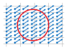
Example. Compute the flux of a constant vector field, $V=<-1,2>$, across a straight line, the segment from $(0,0)$ to $(1,3)$. First parametrize the curve and find its derivative: $$X(t)=<1,3>t,\ 0\le t\le 1,\ \Longrightarrow\ X'(t)=<1,3>\ \Longrightarrow\ X'(t)^\perp=<-3,1>.$$ Then, $$L=\int_CV\, dX^\perp=\int_a^bV(X(t))\cdot X'(t)^\perp\, dt=\int_0^1<-1,2>\cdot <-3,1>\, dt=\int_0^1 5\, dt=5.$$ $\square$

Example. Compute the flux of the radial vector field, $V(X)=X=<x,y>$, across the upper half-circle from $(1,0)$ to $(-1,0)$. First parametrize the curve and find its derivative: $$X(t)=<\cos t,\sin t >,\ 0\le t\le \pi,\ \Longrightarrow\ X'(t)=<-\sin t,\cos t>\ \Longrightarrow\ X'(t)^\perp=<-\cos t,-\sin t>.$$ Then, $$\begin{array}{lll} W&=\int_CV\, dX^\perp=\int_a^bV(X(t))\cdot X'(t)^\perp\, dt\\ &=\int_0^\pi <\cos t,\sin t >\cdot <-\cos t,-\sin t>\, dt\\ &=-\int_0^\pi 1\, dt\\ &=-\pi. \end{array}$$ $\square$

Theorem. The flux is independent of parametrization.

Theorem. $$\int_{-C}V\, dX^\perp=-\int_CV\, dX^\perp.$$

Example. Is the flux positive or negative?

More below:

File:Estimate flux across a curve.png

$\square$

Exercise. Finish the example.

Exercise. What is the value of the line integral of the gradient of a function across one of its level curves?

Theorem (Linearity). For any two vector fields $V$ and $W$ and any two numbers $\lambda$ and $\mu$, we have: $$\int_{C}(\lambda V+\mu W)\, dX^\perp=\lambda\int_CV\, dX^\perp+\mu\int_{C}W\, dX^\perp.$$

Theorem (Additivity). For any two oriented curves $C$ and $K$ that have only finitely many points in common and together form a oriented curve $C\cup K$, we have: $$\int_{C\cup K}V\, dX^\perp=\int_CV\, dX^\perp+\int_KV\, dX^\perp.$$

To study $3$-dimensional flows, we will need to use parametric surfaces.

We can use this construction to model flows across, instead of an imaginary front, a physical barrier. Such a barrier may have a permeability that varies with location. The permeability may also depend on the direction of the flow.

Now, line integrals across closed curves.

Example. What is the work of a constant vector field along a closed curve such as a circle?

Consider two diametrically opposite points. The directions of the tangents to the curve are opposite while the vector field is the same. Therefore, the terms $F\cdot N$ in the work integral are negative of each other. So, because of this symmetry, two opposite halves of the circle will have work negative of each other and cancel. The work is flux! Let's confirm this for $F=<p,q>$ and the standard parametrization of the circle: $$\begin{array}{ll} L&=\oint_CF\, dX^\perp=\int_a^bF(X(t))\cdot X'(t)^\perp\, dt\\ &=\int_0^{2\pi}<p,q>\cdot <-\sin t,\cos t>^\perp\, dt\\ &=\int_0^{2\pi}<p,q>\cdot <-\cos t,-\sin t>\, dt\\ &=\int_0^{2\pi}(-p\cos t-q\sin t)\, dt\\ &=0+0=0. \end{array}$$ There is as much water coming in as going out! $\square$

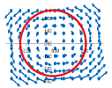
Example. The story is the exact opposite for the rotation vector field: $$F=<-y,x>.$$

Consider any point. The direction of the tangents to the curve is the same as the vector field. Therefore, flux is not zero! Let's confirm this result: $$\begin{array}{ll} L&=\oint_CF\, dX^\perp=\int_a^bF(X(t))\cdot X'(t)^\perp\, dt\\ &=\int_0^{2\pi}<-\sin t,\cos t>\cdot <-\sin t,\cos t>^\perp\, dt\\ &=\int_0^{2\pi}<-\sin t,\cos t>\cdot <-\cos t,-\sin t>\, dt\\ &=\int_0^{2\pi}(\sin t\cos t+\cos t(-\sin t))\, dt\\ &=0. \end{array}$$ No water gets in or out! $\square$