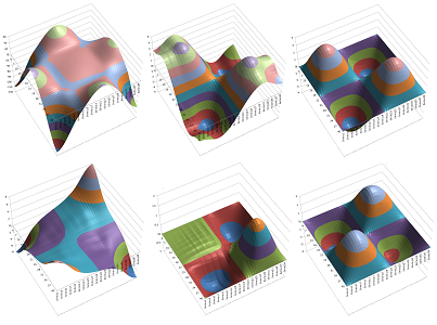
This site is being phased out.
Partial differential equations
Contents
- 1 Heat transfer in dimension $1$: a rod
- 2 The heat equation with respect to difference quotients
- 3 The heat equation with respect to derivatives
- 4 Heat transfer in dimension $2$: a plate
- 5 Wave propagation in dimension $1$: springs and strings
- 6 The wave equation with respect to derivatives
- 7 Wave propagation in dimension $2$: a membrane
Heat transfer in dimension $1$: a rod
In this chapter we will investigate processes that happens -- separately but not independently -- throughout a certain area.
We start in this section with heat transfer within a metal rod.
The rod is seen as split into pieces as if they are separate compartments: the heat is contained in a row of rooms and each room exchanges the material with its two neighbors through its walls.
Suppose
- $a=AB$ is one of the rooms;
- $b,c$ are the two adjacent rooms, left and right;
- $A,B$ are the walls of $a$, left and right.
What makes this different from ODEs is that the functions will have two variables -- with respect to location and with respect to time. The amount of heat $u=u(t,a)$ is simply a number assigned to each room $a$. This is a discrete $1$-form with respect to location $x$ and a $0$-form with respect to time $t$.
A careful look reveals that to model heat transfer, we need to separately record the exchange of heat with each of the adjacent rooms.
The process we are to study obeys the following familiar law of physics.
Newton's Law of Cooling: The rate of cooling of an object is proportional to the difference between its temperature and the temperature an adjacent object.
Of course, cooling means heating when the temperature of the other object is higher.
Our initial assumption is that all rooms have equal size. It follows that the amount of heat in the rooms is proportional to their respective temperatures. This is why we can understand the law of cooling as: the rate of heat transfer between every two adjacent rooms is proportional to the difference between the amounts of heat in them.
Furthermore, what is the magnitude of this rate? It may be slow and it may be fast but it cannot be so fast that the updated value of the heat of the room surpasses that of the other! In order to avoid this “overshoot”, the increment of the heat shouldn't be more that half-distance to the heat of the other room.
This law is nothing but a version of the ODE of population growth and decay except this time each cell has two adjacent cells and two differences are to be taken into account.
The assumption of conservation of energy in room $a$ gives us the following. The change of the amount of the heat in room $a$ over the time increment is equal to $$u(t+1,a)- u(t,a)=-\bigg( \text{ sum of the outflow } g \text{ across the walls of } a\bigg).$$ The outflow gives the amount of flow across a node (from the room to its neighbor) per unit of time. Specifically, the flow is positive at $A$ if it is from left to right and the opposite for $B$; then: $$u(t+1,a)- u(t,a)=-\big( g(A,t)-g(B,t) \big) = g(A,t)-g(B,t).$$
Now, we need to express $g$ in terms of $u$. The flow $g(A)$ through wall $A$ of room $a$ is proportional to the difference of the amounts of heat in $a$ and the other room adjacent to $A$. So, $$\begin{array}{lll} g(A,t) &= - k(A) \big( u(t,a) - u(t,b) \big),\\ g(B,t) &= - k(B) \big( u(t,c) - u(t,a) \big). \end{array}$$ Here, $k(A) \ge 0$ represents the permeability of the wall $A$ at a given time over the same time period. This is a $0$-form.
Exercise. Can $k$ also depend on $t$?
The result of the substitution is the following equation: $$u(t+1,a)- u(t,a) = \Big[- k(A) \big( u(t,a) - u(t,b)\big)\Big] - \Big[- k(B) \big( u(t,c) - u(t,a)\big)\Big]. $$ Let's make $b$ and $c$ specific: $$b=a-1,\ c=a+1.$$ Then the right-hand side becomes the increment in the recursive formula for the simulation: $$u(t+1,a)= u(t,a) + \Big[- k(A) \big( u(t,a) - u(t,a-1)\big) + k(A+1) \big( u(t,a+1) - u(t,a)\big)\Big].$$
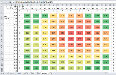
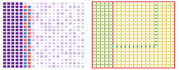
Suppose our rod is split into ten pieces as if they are separate compartments as explained above. Each of them is represented by a (wider) cell in the spreadsheet. This is what you see at the top of the spreadsheet below. The walls of the compartments are shown as (narrower) cells.
The time axis is vertical.
Now, each of the cells representing the compartments contains a number which is the amount of heat $u$ at that location at that time. Next, each of the cells representing the walls contains a number which is the permeability $k$ at that location at that time. The heat flow across the walls is computed according to the formula discussed above and the new value of $u$ is computed every time we move to the next row.
The spreadsheet formula is: $$\texttt{=R[-1]C-RC[-1]*(R[-1]C-R[-1]C[-2])+RC[1]*(R[-1]C[2]-R[-1]C) }.$$ This is the dependence diagram of the formula:
There are two main cases.
Example (insulated rod). Suppose we put insulators to the ends of our rod and suppose they have initially a lower temperature than that of the rod. The areas adjacent to the ends quickly cools down. At this point we start our simulation. Heat transfer continues within the body of the rod with virtually no transfer through the insulators.
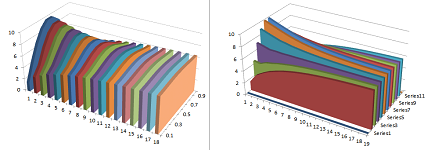
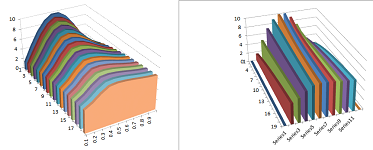
We set the initial value of $u$ to go from $0$ to $1$ and then back to $0$ at the other end. For example, we may have: $$u(0,x)=10\sin (\pi x).$$ The permeability is zero at the ends and non-zero throughout the rest of the rod. For example, we may have: $$k(0)=k(1)=0 \text{ and } k(x)=.45 \text{ for } 0<x<1.$$ This is the result of our simulation is the collection of graphs of the function $u(t,\cdot)$ of one variable for each $t$ (the graph of $u$ is of course a surface):
Above we see either the distribution of heat throughout the rod at every moment of time or the dynamics of the temperature at every location. Conclusion: the temperature evens out! Note that the total amount of heat in the rod remains the same (seen under “total” in the spreadsheet shown above).
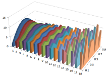
As a warning, if we choose our coefficient of permeability larger than $1/2$, the simulation fails quickly:
$\square$
Example (heated rod). Suppose our rod is inserted to fix a gap in a long pipe with warmer temperature. Once in, the areas adjacent to the ends of the rod start to exchange heat with the pipe. However, the effect on the pipe's temperature is negligible. At this point we start our simulation.
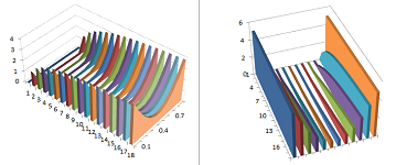
We set the initial value of $u$ to be $0$ throughout the rod while the outside temperature is $5$. The permeability is $.45$ throughout the rod. This is the result of our simulation:
The temperature evens out!
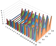
If we choose our coefficient of permeability larger than $1/2$, the simulation fails quickly:
$\square$
Exercise. What kind of curve do we see at the edge ($x=0$) of this surface?
The heat equation with respect to difference quotients
We start with a more general model for heat transfer in a rod. This time, the cell sizes may vary and so do the lengths of the intervals of time.
What makes this different from ODEs is that the functions will have two variables -- with respect to location and with respect to time. Our function $u=u(t,x)$ represents the amount of heat or material at location $x$ at time $t$. The result is a partial differential equation (PDE) derived below.
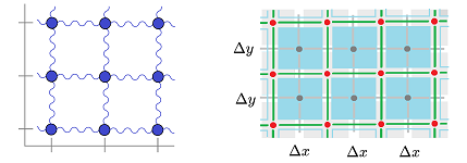
The interpretation is dual to the one above: instead of rooms and walls between them, we speak of containers and pipes between them respectively. This correspondence is illustrated below:
As a result, our function $u$ will be defined at the end-points of the intervals.
Let's first review the material about the partial differences and difference quotients.
We start with partitions in the $x$- and the $t$-axes:
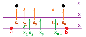
A partition of the interval $[a,b]$ in the $x$-axis consists of $n+1$ nodes: $$a=x_{0},\ x_{1},\ x_{2},\ ...,\ x_{n-1},\ x_{n}=b,$$ and $n$ secondary nodes in between: $$s_{1},\ s_{2},\ ...,\ s_{n-1},\ s_{n},$$ with the increments: $$\Delta x_i = x_i-x_{i-1},\ i=1,2,...,n.$$ A partition the interval $[c,d]$ in the $t$-axis consists of $m+1$ nodes: $$ c=t_{0},\ t_{1},\ t_{2},\ ... ,\ t_{m-1},\ t_{m}=d,$$ and $m$ secondary nodes in between: $$ q_{1},\ q_{2},\ ... ,\ q_{m-1},\ q_{m},$$ with the increments: $$\Delta t_i = t_i-t_{i-1},\ i=1,2,...,m.$$
We use those construct a partition $P$ of a rectangle $R=[a,b]\times [c,d]$ in the $xt$-plane. The lines $x=x_i$ and $t=t_j$ cut the rectangle $[a,b]\times [c,d]$ into smaller rectangles $[x_{i},x_{i+1}]\times [t_{j},t_{j+1}]$.
We will also need the secondary nodes of partition $P$ that are located at each of the horizontal and vertical edges; for each pair $i=1,2,...,n$ and $j=0,1,2,...,m$, we have:
- a point $S_{ij}=(s_{i},t_j)$ in the segment $[x_{i},x_{i+1}]\times \{t_{j}\}$,
and for each pair $i=0,1,2,...,n$ and $j=1,2,...,m$, we have:
- a point $Q_{ij}=(x_i,q_{j})$ in the segment $\{x_{i}\}\times [t_{j},t_{j+1}]$.
Now, suppose $u(t,x)$ represents the amount of heat in compartment $x$ -- a node on the $x$-axis -- at time $t$ -- a node on the $t$-axis. Then $u$ is defined at the nodes of the partition of the rectangle. It is then a $0$-form (with respect to both $x$ and $t$).
The partial differences of $u$ with respect to $x$ and $t$ are defined at these secondary nodes of the partition by the following (omitting indices): $$\Delta_x u\, (t,s)=u(t,x+\Delta x)-u(t,x) \text{ and } \Delta_t u\, (q,x)=u(t+\Delta t,x)-u(t,x);$$ and the difference quotients are defined by: $$\frac{\Delta u}{\Delta x}(t,s)=\frac{u(t,x+\Delta x)-u(t,x)}{\Delta x} \text{ and } \frac{\Delta u}{\Delta t}(q,x)=\frac{u(t+\Delta t,x)-u(t,x)}{\Delta t}.$$
Now back to the rod. Suppose the amount of flow (left to right) of heat or material along the pipe $[x_{k-1},x_k]$ during a period of time $[t_{j-1},t_j]$ is denoted by $g=g(q_{j},s_{k})$.
The assumption of conservation of energy (or material) gives us the following:
- the change of the amount of the heat in compartment $x$ over a given interval of time is equal to the sum -- accounting for the directions -- of the flow along the two pipes that leave $x$.
Then, $$\Delta_t u\, (q_{j},x_{i})= g(q_{j},s_{i-1})-g(q_{j},s_{i}).$$
Next, we separately record the exchange of heat between each pair of adjacent compartments according to the Newton's Law of Cooling: the rate of cooling of an object is proportional to the difference between its temperature and the temperature of the adjacent object. So, in addition to the amount of heat (or material), we need to include the temperature (or the density of the material) in our analysis! Of course, the latter is simply the former divided by the size of the compartment. Where does that come from?
We consider the secondary partition in the $x$-axis:
The idea is that the length of the interval $[s_{k-1},s_k]$ in the dual partition corresponds to the size of the compartment $x_k$: $$\Delta s_k=s_k-s_{k-1}.$$
Suppose $w=w(t_j,x_k)$ is the temperature of compartment $x_k$ at time $t_j$. Then we have a relation: $$u(t_j,x_k)=w(t_j,x_k)\Delta s_k.$$
Now, the law of cooling takes the following form:
- 1. the flow of heat (during a period of time) along a pipe is proportional to the difference of the temperature in the two compartments at the two ends of the pipe (in the beginning of the period of time).
Furthermore, it is natural to assume that
- 2. the flow is proportional to the length of the period of time, and
- 3. the flow is inversely proportional to the length of the pipe.
So, $g(s_i,q_j)$ is proportional to these three quantities:
- 1. $w(t_j,x_{i}) - w(t_j,x_{i-1})=\Delta_x w\, (t_j,s_{i})$,
- 2. $\Delta t_j$,
- 3. $\frac{1}{\Delta s_i}$.
In other words, $$g(q_j,s_i)=- k(t_j,s_{i})\Delta t_j\frac{1}{\Delta s_i}\Delta_x w\, (t_{j},s_{i}),$$ where the coefficient $k(t_j,s_i) \ge 0$ represents the permeability of the pipe $[x_{i-1},x_i]$ at time $t_j$. It is a $1$-form with respect to $x$ and a $0$-form with respect to $t$. We now apply this formula to the two pipes that leave compartment $x_i$, over the period of time $[t_{j-1},t_j]$: $$\begin{array}{lll} g(t_j,s_{i-1}) &= - k(t_j,s_{i-1})& \Delta t_j & \frac{1}{\Delta s_{i-1}} & \Delta_x w\, (t_j,s_{i-1}),\\ g(t_j,s_i) &= - k(t_j,s_i) & \Delta t_j & \frac{1}{\Delta s_i} & \Delta_x w\, (t_j,s_{i}). \end{array}$$
We substitute these two into the conservation formula above and the result is the following: $$\Delta_t u\, (q_j,x_i)= g(s_{i-1})-g(s_{i}) = \Delta t_j\Big( - k(q_j,s_{i-1}) \frac{\Delta w}{\Delta x}(s_{i-1},t_{j}) + k(q_j,s_i) \frac{\Delta w}{\Delta x}(q_j,s_{i})\Big). $$ We substitute the temperature $w$ into the left-hand side: $$\Delta_t u\, (q_j,x_i)=\Delta_t w\, (q_j,x_i)\Delta s_i,$$ and obtain the following: $$\frac{\Delta w}{\Delta t}(q_j,x_i)= \frac{1}{\Delta s_i}\Big( - k(q_j,s_{i-1}) \frac{\Delta w}{\Delta x}(t_j,s_{i-1}) + k(q_j,s_i) \frac{\Delta w}{\Delta x}(q_j,s_{i})\Big). $$ The expression in the parentheses is simply the difference of the function $k\frac{\Delta w}{\Delta x}$. So, we have the discrete heat equation: $$\frac{\Delta w}{\Delta t}(q_j,x_i)=\frac{\Delta \big(k\frac{\Delta w}{\Delta x}\big)}{\Delta x}(t_j,x_i).$$ When $k$ is constant, we can use the second differences introduced in Chapter 18: $$\begin{array}{|c|}\hline\\ \quad \frac{\Delta w}{\Delta t}=k\frac{\Delta^2 w}{\Delta x^2}. \quad \\ \\ \hline\end{array} $$ We should keep in mind that the left-hand side is defined at the vertical secondary nodes and the right-hand side at the primary nodes of the partition of the rectangle.
The incremental formula produced is a generalization of the one in the last section: $$w(q_j,x_i)=w(q_{j-1},x_i)+\frac{\Delta \big(k\frac{\Delta w}{\Delta x}\big)}{\Delta x}(t_j,x_i)\Delta t_j.$$
Example (heated rod). What will happen to the rod heated at the ends when the permeability varies? The initial temperature is still $0$ while the outside temperature is $5$. The permeability will remain $.45$ throughout the half of the rod and $.1$ on the left. This is the result of our simulation:
The temperature evens out again but, predictably, the left end is falling behind! $\square$
Exercise. What if the permeability varies with time?
Exercise. What if the permeability of each wall is proportional to the average temperature of the two adjacent compartments?
The heat equation with respect to derivatives
We now consider the continuous case of heat transfer.
Suppose the temperature function $w$ is defined for all $x$ and $t$ within some open subset $U$ of the plane and it is sampled at the nodes of a partition of rectangle $[0,b]\times [0,d]$ contained in that subset. We refine this partition of the rectangle and take the limit of the discrete heat equation with constant permeability $k$, $$\frac{\Delta w}{\Delta t}(q_j,x_i)=k\frac{\Delta^2 w}{\Delta x^2}(t_j,x_i), $$ as $\Delta x\to 0$ and $\Delta t\to 0$. We have the heat equation: $$\begin{array}{|c|}\hline\quad \frac{\partial w}{\partial t}=k\frac{\partial ^2 w}{\partial x^2}. \quad \\ \hline\end{array} $$
A solution $w$ of this partial differential equation (PDE) is a function
- defined and continuous on the rectangle,
- differentiable with respect to $t$ inside of it, and
- twice differentiable with respect to $x$ inside the rectangle, such that
- the equation is satisfied for each pair $(x,t)$ such that $x$ is in $(0,b)$ and $t$ is in $(0,d)$.
Because this is a function of two variables, a solution is made specific by a combination of:
- the initial condition, providing the values of $w(0,x)$ in the beginning, such as:
$$w(0,x) = f(x), \quad \text{ when } 0\le x \le b;$$ where the function $f$ is given, and
- the boundary condition, providing the values of $w$ at the ends of the rod, such as:
$$w(t,0) = 0 = w(t,b), \quad \text{ when } 0\le t \le d,$$ which is the zero boundary condition.
In contrast to our study of ODEs, here we won't search for solutions for all possible initial conditions. We will deal with this question: is it possible that $u$ is the result of multiplication of $f$ by some numbers that depends on $t$? Let's assume: $$ w(t,x) = f(x) T(t).$$ The idea is similar to that of separation of variables for ODEs presented in Chapter 23. Substituting $w$ into the PDE gives us the following: $$\frac{T'(t)}{k T(t)} = \frac{f' '(x)}{f(x)}.$$ Since the right hand side depends only on $x$ and the left hand side only on $t$, both sides have to be equal to some constant number, say $−\lambda$. We have: $$T'(t) = - \lambda\, k\, T(t);$$ and $$f' '(x) = - \lambda\, f(x).$$
We can solve these ODEs. The result depends on the sign of $\lambda$.
Case 1: $\lambda < 0$. Then, $$f(x) = B e^{\sqrt{-\lambda} \, x} + C e^{-\sqrt{-\lambda} \, x},$$ for some $A,B,C$.
Exercise. Show that from the boundary conditions it follows that $A=B=C=0$.
Exercise. Draw the same conclusion for Case 2: $\lambda =0$.
We are left with Case 3: $\lambda >0$. From a certain result in Chapter 23, it follows that $$T(t) = A e^{-\lambda k t}$$ and $$f(x) = B \sin(\sqrt{\lambda} \, x) + C \cos(\sqrt{\lambda} \, x),$$ for some constant $A,B,C$. They are found from the initial conditions: $$w(0,x)=f(x) T(0) = f(x)\ \Longrightarrow\ T(0)=1\ \Longrightarrow\ A=1;$$ and boundary conditions: $$w(0,t) = f(0) T(t)=0 \ \Longrightarrow\ f(0)=0 \ \Longrightarrow\ B \sin(\sqrt{\lambda} \, 0) + C \cos(\sqrt{\lambda} \, 0)=0 \ \Longrightarrow\ C=0,$$ and $$w(t,b) = f(b) T(t)=0 \ \Longrightarrow\ f(b)=0 \ \Longrightarrow\ B \sin(\sqrt{\lambda} \, b) + 0 \cos(\sqrt{\lambda} \, b)=0 \ \Longrightarrow\ \sqrt{\lambda} \, b=\pi n,$$ for some integer $n$.
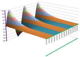
Theorem. If $$\sqrt{\lambda} =\pi n/b$$ for some integer $n$, then there is a solution to the heat equation with the zero boundary condition: $$w(t,x)=Be^{-\lambda k t} \sin(\sqrt{\lambda} \, x).$$
Example. The function above is plotted below:
$\square$
Corollary. The sum of solutions of the heat equation is a solution of the heat equation; therefore, $$w(t,x)=\sum_{n=1}^N B_ne^{-\lambda_n k t} \sin(\sqrt{\lambda_n} \, x),$$ where $$\sqrt{\lambda_n} =\pi n/b,\ n=1,2,...,N,$$ is a solution of the heat equation.
Exercise. Prove the corollary.
Heat transfer in dimension $2$: a plate
Heat transfer exhibits a dispersal pattern with no particular direction:
The heat is exchanged -- with adjacent locations. The pattern created is a sequence of concentric circles. The process is also known as diffusion.
To model heat propagation, imagine a grid of square rooms and the temperature of each room changes by a proportion of the average of the temperature of the four adjacent rooms. Its spreadsheet simulation is given by the following short formula: $$\texttt{= RC - .25*k*( (RC-RC[-1]) + (RC-RC[1]) + (RC-R[-1]C) + (RC-R[1]C) )}$$ Only a proportion, $k$, dependent on the presumed length of the time interval, of the total amount is exchanged.
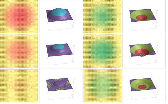
Example (a drop diffused). The two images below are the initial state -- a single initial hot spot or a drop of liquid -- and the results after $1,700$ iterations of such a simulation for $h=.01$ (the value at the border fixed at $0$):
$\square$
Example (a source of heat). On a larger scale, the simulation produces a realistic circular pattern even though it starts straight. Below we have a single-point but permanent source of heat shown after $3$ and then after $3000$ iterations:
$\square$
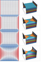
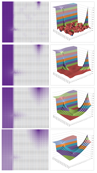
Example (heater). For each $t$, our function $u(t,\cdot,\cdot)$ is a function of two variables and can be visualized by its graph. For example, a square heater in the middle of a room will produce the following dynamics of distribution of the temperature over the floor:
$\square$
Example (walls). Two opposite walls of a room are worm and the other two are cold. The temperature develops into a saddle-like pattern:
$\square$
Warning: One needs to use an extra sheet (as a buffer); otherwise spreadsheet's sequential -- cell-by-cell in each row and then row-by-row -- manner of evaluation will cause a skewed pattern:
Example. Implement the above examples.
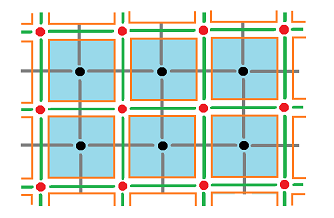
Thus, we have four walls of the room or, dually, four pipes leaving the room and that is how the heat (or material) is exchanged with the neighbors. This correspondence is illustrated below.
The latter interpretation is preferable because our temperature distribution function $w$ is then a $0$-form in a space of any dimension.
In contrast to the above simulations, for the general case, we will take into account the permeability of the walls/pipes.
Recall that a partition of a box $B$ in the $txy$-space comes from partitions of its three edges as described in Chapter 20: $$\begin{array}{lll} t_{0}&q_1& t_{1}&q_2& t_{2}&q_3& ...;\\ x_{0}&s_1& x_{1}&s_2& x_{2}&s_3& ...;\\ y_{0}&p_1& y_{1}&p_2& y_{2}&p_3& ....\\ \end{array}$$
We make a simplifying assumption that all compartments have equal sizes. Then, for compartment located at $(x_i,y_j)$, this is the total inflow: $$\begin{array}{ccccc} \bullet& -K(t_k,s_{i},y_{j-1}) \Delta_yu\, (t_k,s_{i},p_{j-1})&\bullet\\ - K(t_k,s_{i-1},y_j) \Delta_x u\, (t_k,s_{i-1},y_j)&& + K(t_k,s_i,y_j) \Delta_x u\, (t_k,s_{i},y_j)\\ \bullet& +K(t_k,s_{i},y_{j}) \Delta_y u\, (t_k,s_{i},p_{j})&\bullet \end{array}.$$ The four terms are the inflows across each of the four walls of the compartment and they are arranged accordingly. The proportion of the heat exchanged across each wall is given by the function $K\ge 0$. It incorporates the permeability of the walls, their sizes, the length of the time interval, and so on.
The difference equation for the heat, or temperature, $u=u(t,x,y)$ is the following: $$\Delta_t u\, (q_{k},x_i,y_j)= \text{ total inflow },$$ and the recursive formula to be implemented is simply: $$u(t_k,x_i,y_j)=u(t_{k-1},x_i,y_j)+\text{ total inflow }.$$
The spreadsheet consists of several sheets computed consecutively:
- the permeability for each wall,
- the initial temperature for each compartment,
- the buffer (copied current values),
- the difference and the flow of temperature for each wall,
- the total flow for each compartment, and finally
- the current values of the temperature.
The last formula is: $$\text{the current value = the buffer value + the total inflow }.$$
As you can see, the square cells represent the compartments and the narrow ones the walls.
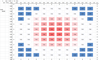
Example (coffee). Suppose coffee is poured into an insulated cup. The temperature of the areas adjacent to the sides of the cup quickly cools down. At this point we start our simulation. These are the first two sheets: the permeability (zero around the edge of the cup) and the initial temperature (hot inside, cold outside):
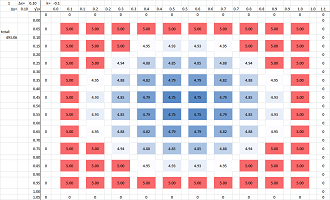
Heat transfer continues within the body of the coffee with virtually no transfer through the walls of the cup. These are the results after $50$ iterations:
One can see that the total amount of heat is preserved. $\square$
Example (soda). Suppose a can of soda is taken out of the refrigerator. The areas adjacent to the sides of the can start to exchange heat with the outside. However, the effect on the outside temperature is negligible. At this point we start our simulation. These are the first two sheets: the permeability (high throughout) and the initial temperature (cold inside, hot outside):
The temperature outside the can remains unchanged! These are the results after $50$ iterations:
$\square$
Exercise. What if the permeability of a wall is proportional to the average temperature of the two adjacent compartments?
When $K$ is constant as another simplifying assumption, the right-hand side of our equation becomes recognizable: $$\begin{array}{ll} \Delta_t u\, (q_k,x_i,y_j)&= K\left( \begin{array}{ccccc} \bullet& -\Delta_yu\, (t_k,s_{i},p_{j-1})&\bullet\\ - \Delta_x u\, (t_k,s_{i-1},y_j)&& + \Delta_x u\, (t_k,s_{i},y_j)\\ \bullet&+\Delta_y u\, (t_k,s_{i},p_{j})&\bullet \end{array}\right)\\ &=K\Big(\big[\Delta_x u\, (t_k,s_{i},y_j)-\Delta_x u\, (t_k,s_{i-1},y_j)\big]+\big[\Delta_y u\, (t_k,s_{i},p_{j})-\Delta_yu\, (t_k,s_{i},p_{j-1})\big]\Big)\\ &=K\big(\Delta_x\Delta_x u\, (t_k,x_{i},y_j)+\Delta_y\Delta_y u\, (t_k,x_{i},y_j)\big)\\ &=K\big(\Delta_x^2 u\, (t_k,x_{i},y_j)+\Delta_y^2 u\, (t_k,x_{i},y_j)\big). \end{array}$$ These are the second differences introduced in Chapter 18. Our partial difference equation becomes the following: $$\Delta_t u=K\left(\Delta_x^2 u+\Delta_y^2 u\right).$$
Exercise. Derive a version of this equation for a variable $K$.
When $u$ is defined throughout the region, the difference equation corresponds to the heat equation for partial derivatives: $$\frac{\partial u}{\partial t}=\alpha\left(\frac{\partial^2 u}{\partial x^2}+\frac{\partial^2 u}{\partial y^2}\right),$$ with the last expression called the Laplace operator of $u$.
Exercise. Derive this equation from the last.
Exercise. Find a solution of the form $u(t,x,y)=(X(x)+Y(y))T(t)$.
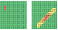
Example (migration). The discrete heat equation can also be used to model moving populations. Indeed, it is conceivable that people migrate from their current location to an adjacent area with a lower population density. Below we imagine two areas in a country: one is densely and uniformly populated ($u(0,x,y)=1$) and the other thinly and randomly ($u(0,x,y)$ close to $0$). The two parts are separated by a river ($k=0$). Now a bridge is built over the river as well a road ($k=1$) from the bridge to a town on a city on the other end of the country. The initial distribution of the population is shown on the left and the permeability is shown on the right:
At this point people start to cross the river and spread into the thinly populated area -- especially along the road. We also imagine that the city is a constant source of new settlers arriving from the outside, $u(t,x_0,y_0)=1$.
$\square$
Exercise. (a) Incorporate into the model the possibility of growing population with location-dependent rates. (b) Incorporate into the model the possibility of sustainability limits (location-dependent) on the population growth. Derive the PDE.
Example (diffusion in a flow). If we drop dye in a liquid, it will diffuse according to the heat equation. What if the liquid is in motion? Let's see what happens if we let a drop of dye to be taken by a flow. As a simple example, we follow the rule that:
- the amount of dye in each cell is split and passed to the adjacent cells along the vectors of the vector field proportional to the values attached to the edges.
For example, we can choose $1$'s on the horizontal edges and $0$s on the vertical edges. Then the flow will be purely horizontal. If we reverse the values, it will be purely vertical. Now what if we choose $1$'s on both vertical and horizontal edges? $$ \newcommand{\ra}[1]{\!\!\!\!\!\!\!\xrightarrow{\quad#1\quad}\!\!\!\!\!} \newcommand{\da}[1]{\left\downarrow{\scriptstyle#1}\vphantom{\displaystyle\int_0^1}\right.} \newcommand{\la}[1]{\!\!\!\!\!\!\!\xleftarrow{\quad#1\quad}\!\!\!\!\!} \newcommand{\ua}[1]{\left\uparrow{\scriptstyle#1}\vphantom{\displaystyle\int_0^1}\right.} % \begin{array}{cccccccccccccccccc} & &\ \da{1} & & \ \da{1} & & \ \da{1} \\ & \ra{1} & \bullet & \ra{1} & \bullet & \ra{1} & \bullet & \ra{1}\\ & &\ \da{1} & &\ \da{1} & & \ \da{1} \\ & \ra{1} & \bullet & \ra{1} & \bullet & \ra{1} & \bullet & \ra{1}\\ & &\ \da{1} & & \ \da{1} & & \ \da{1} \end{array}$$ It is simple: the amount of dye in each cell is split in half and passed to the two adjacent cells along the vectors. The liquid is flowing down and right equally. We see some dispersal, but the predominantly diagonal direction of the spreading of the dye is also evident:
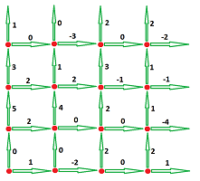
A more general example is this. Imagine that a liquid moves along the square grid which is thought of as a system of pipes:
In the picture above, the numbers represent “flows” through these “pipes”, with the direction determined by the direction of the $x,y$-axes. In particular,
- the “$1$” can be understood as: “$1$ cubic foot per second from left to right”.
- the “$2$” can be understood as: “$2$ cubic feet per second upward”.
However, for the sake of conservation of matter, these numbers have to be normalized. Then $1/3$ of the amount goes right and $2/3$ goes up. Of course, we this is a discrete $1$-form. $\square$
Exercise. Create a spreadsheet and confirm the pattern. What happens if the flow takes horizontally twice as much material as vertically?
Wave propagation in dimension $1$: springs and strings
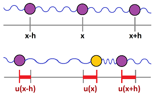
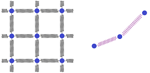
Previously, we studied the motion of an object attached to a wall by a (mass-less) spring. Imagine this time a string of objects connected to each other with springs:
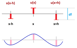
Let $u=u(t,x)$ measure the displacement from the equilibrium of the object associated with position $x$ at time $t$. The partitions for $x$ and $t$ are the same as in the beginning of the chapter.
First, we consider the spatial variable, $x$. Each object is located at a primary node of the partition with a (possibly variable) distance $h=\Delta x$ to its neighbor and the distance between the secondary nodes is $\Delta s$.
According to Hooke's law, the force exerted by the spring is: $$H = -k S,$$ where $S$ is the change of the length of the spring from its equilibrium state and the constant, stiffness, $k$ reflects the physical properties of the spring. Then, if this is the spring that connects locations $x_{p-1}$ and $x_p$, its compression is the difference of the displacements of the two objects. In other words, we have: $$S=u(t_j,x_{p-1}) - u(t_j,x_p).$$ Therefore, the force of this spring is $$H_{p} = k(t_j,s_p) \left[ u(t_j,x_{p-1}) - u(t_j,x_p) \right]=-k(t_j,s_p) \Delta_x u\, (t_j,s_{p})=-(k \Delta_x u) (t_j,s_{p}),$$ where $k$ is the location- and time-dependent stiffness of the springs.
This formula, $$H_{p} =-(k \Delta_x u) (t_j,s_{p}),$$ expresses the force affecting an object at some location in terms of some quantity that depends on both location and time. It has other interpretations that depend on interpretations of $u$.
Let's consider an oscillating string:
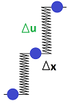
Here, the pieces of the string are vertically displaced (that's $\Delta_x u$) while the waves propagate horizontally. At its simplest, we have a collection of weights that can move only vertically connected by vertical springs:
The horizontal distance between objects, $\Delta x$, remain unchanged while the height, $u(t,x)$, varies with time. The vertical displacement is $\Delta_x u$. Applying Hooke's law again, we find the exactly the same formula for the force exerted by the spring: $$H = -k \Delta_x u.$$
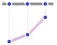
A more complex model is the following. We still imagine that the string is made of springs with weights but the spring can go diagonally:
As you can see, the horizontal distance between the weights still remains unchanged; that's $\Delta x$. Just as before, we use Hook's Law: the force exerted by the spring is $F = -k S$, where $S$ is the change of the length of the spring from its non-stretched state and $k$ is the stiffness of this spring.
We assume that the equilibrium state of each spring is $0$. Then $S$ is simply the distance between the two weights. Suppose $H$ is the vertical component of the force $F$. Examining similar triangles reveals: $$\frac{F}{H}=\frac{S}{\Delta_x u}.$$ Therefore, $$\frac{-k S}{H}=\frac{S}{\Delta_x u},$$ then $$H=-k\Delta_x u.$$ The equation is identical to the one for the previous approach!
From this equation we derive the differential equation that governs these waves modeled by any of these three approaches.
Let $F(x_i,t_j)$ be the force that acted on the object located at $x_i$ at time $t_j$. There are two Hooke's forces acting on this object from the two adjacent springs: $H_{i-1}$ and $H_{i}$, pulling in the opposite directions. Therefore, we have: $$\begin{array}{lll} F(x_i,t_j) &= H_{i-1} &- H_{i} \\ &=-(k\Delta_x u)(t_j,s_{i-1})&+(k\Delta_x u)(t_j,s_i)\\ &=\Delta_x(k\Delta_x u)(t_j,x_i). \end{array}$$ Note that this is the same expression as in the right-hand side of the heat equation!
Second, we consider the temporal variable, $t$. Each increment $\Delta t$ and $\Delta q$ of time may have a different duration. Now suppose that the object located at $x_i$ has mass $m(x_i)$. Then, by the Second Newton's Law (Chapter 8), the total force is $$F(t_j,x_i)=m(x_i)a(t_j,x_i),$$ where $a(t_j,x_i)$ is the acceleration of object $x_i$ at time $t_j$. As we know, this is the second derivative of the location with respect to time, $$a(t_j,x_i)=\frac{\Delta^2 u}{\Delta t^2}(t_j,x_i).$$
We have now the difference wave equation: $$\begin{array}{|c|} \hline \\ \quad \frac{\Delta^2 u}{\Delta t^2}(t_j,x_i)=\frac{1}{m(x_i)}\Delta_x(k\Delta_x u)(t_j,x_i). \quad \\ \\ \hline \end{array}$$
Now we will derive the recursive formulas in order to simulate wave propagation with a spreadsheet. We make several simplifying assumptions.
First, we assume that the time increments are equal: $\Delta t =\Delta q=1$. Then the left-hand side of our equation is the following: $$m \Delta_t^2 u = m\big( u(t+1,x)-2u(t,x)+u(t-1,x) \big).$$ For the right-hand side, we can use the original expression: $$ \Delta_x (k \Delta_xu) = k \Big[ u(t,x-1) - u(t,x) \Big] + k\Big[ u(t,x+1) - u(t,x) \Big].$$
Second, we assume that $k$ and $m$ are constant. Then just solve for $u(x,t+1)$: $$\begin{array}{ll} u(t+1,x) &= 2u(t,x) - u(t-1,x) + \alpha\Big(u(t,x+1)-2u(t,x)+u(t,x-1)\Big), \end{array}$$ where $$\alpha = \frac{k}{m}.$$
To visualize the formula, we arrange the terms in a table to be implemented as a spreadsheet: $$\begin{array}{l|cccccc} & x-1 & x & x+1\\ \hline t-1 & & -u(t-1,x) \\ t &=\alpha u(t,x-1) & +2(1-\alpha)u(t,x) & +\alpha u(t,x+1)\\ t+1 & & u(t+1,x) \end{array}$$ Even though the right-hand side is the same, the table is different from that of the heat equation. The presence of the second derivative with respect to time makes it necessary to look two steps back, not just one. That's why we have two initial conditions.
We suppose, for simplicity, that $\alpha=1$.
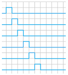
Example. Choosing the simplified settings allows us to easily solve the following initial value problem by hand: $$\begin{array}{lll} \Delta_t^2 u=\Delta_x^2 u;\\ u(t,x)=\begin{cases} 1 &\text{ if } t=0,x=1;\\ 0 &\text{ if } t=0,x\ne 1;\\ 1 &\text{ if } t=1,x=2;\\ 0 &\text{ if } t=1,x\ne 2. \end{cases} \end{array}$$ Initially, the wave has a single bump and then the bump moves one step from left to right. The negative values of $x$ are ignored.
Now, setting $k=1$ makes the middle term in the table disappear. Then every new term is computed by taking an alternating sum of the three terms above, as shown below: $$\begin{array}{l|cccccccc} t \backslash x& 1 & 2 & 3 & 4 & 5 & 6 & 7 & ..\\ \hline 0 & 1 & 0 & 0 & 0 & 0 & [0] & 0 & ..\\ 1 & 0 & 1 & 0 & 0 & [0] & 0 & [0] & ..\\ \hline 2 & 0 & 0 & 1 & 0 & 0 & (0) & 0 & ..\\ 3 & 0 & 0 & 0 & 1 & 0 & 0 & 0 & ..\\ 4 & 0 & 0 & 0 & 0 & 1 & 0 & 0 & ..\\ 5 & 0 & 0 & 0 & 0 & 0 & 1 & 0 & ..\\ .. & .. & .. & .. & .. & .. & .. & .. & .. \end{array}$$ We can see that the wave is a single bump running from left to right at speed $1$:
$\square$
Exercise. Set up and solve an IVP with $2$ bumps, $n$ bumps.
The simplest way to implement this dynamics with a spreadsheet is to use the first two rows for the initial conditions and then add one row for every moment of time. The Excel formula is: $$\texttt{ = R1C5*R[-1]C[-1] + 2*(1-R1C5)*R[-1]C + R1C5*R[-1]C[1] - R[-2]C}$$ Here cell $\texttt{R1C5}$ contains the value of $\alpha$.
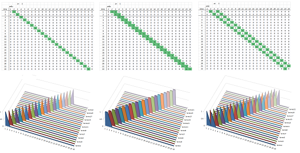
Example (bumps). The simplest propagation pattern is given by $\alpha=1$. Below we show the propagation of a single bump, a two-cell bump, and two bumps:
In the second row, the swing of the wave is visualized as a function of two variables. $\square$
Exercise. Modify the spreadsheet to introduce walls (one and then two) into the picture:
Exercise. Modify the spreadsheet to accommodate non-constant data by adding variability to the following: (a) the stiffness $k$ (shown below), (b) the weights $m$, (c) the space intervals $\Delta x$, (d) the time intervals $\Delta t$.
Exercise. Implement a spreadsheet simulation for the case of non-constant $m$. Hint: you will need two buffers.
Below we consider a rope with fixed ends. This is reflected in the boundary conditions: $$u(t,0)=u(t,n)=0,\ \text{ for all }t.$$ We also choose $\alpha =1$.
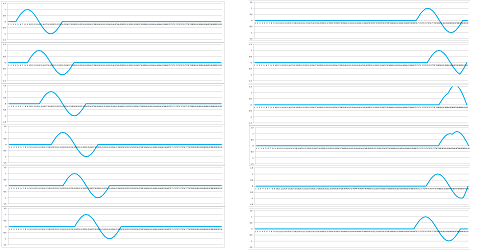
Example (whip). The simulation starts with an arbitrary shape given by the first initial condition $u(0,x)$. It is a small piece of a sinusoid. The second initial condition is just a shift, $u(1,x)=u(0,x-1)$, of the first. The simulation continues to produce this shift at every iteration; in fact, the magnitude of the initial shift is the speed of propagation of the shape. The rope behaves like a whip. This effect is known as a “traveling wave”.
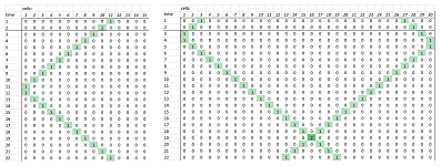
Furthermore, because the end is attached to the wall, the wave bounces off the end. When the coefficient $\alpha$ is $1.01$ instead of $1$, the model breaks down very quickly:
$\square$
Example (vibrating string). The simulation starts with a sinusoid given by the first initial condition $u(x,0)=\sin (\pi x/n)$. The second initial condition is an exact copy, $u(1,x)=u(0,x)$, of the first. The initial velocity, then, is zero (there is of course acceleration). The simulation produces more sinusoids and a perfect vibration:
We can also visualize $u$ by its graph as a function of two variables:
$\square$
Exercise. What if half of the string is made of a stiffer material?
The wave equation with respect to derivatives
We now consider the continuous case of wave propagation.
Suppose the function $u$ is defined for all $x$ and $t$ within some open subset $U$ of the plane and it is sampled at the nodes of a partition of rectangle $[0,b]\times [0,d]$ contained in that subset. We now utilize the results from the last section in the special case of a finite string of weights and springs:
These are our assumptions:
- the array of $N$ identical weights; $m$ is constant,
- the weights are distributed evenly over the length $L= N\Delta x$ of the string,
- the total mass is $M= Nm$,
- the springs are identical; $k$ is constant,
- the total spring constant of the array is $K= k/N$,
- the partition of the string is uniform: $\Delta x =\Delta s=h$,
- the partition of the time interval is also uniform: $\Delta t =\Delta q$.
We can re-write the difference equation for wave propagation from the last section as follows: $$\begin{array}{ll} m\frac{u(t+\Delta t,x)-2u(t,x)+u(t-\Delta t,x) }{ (\Delta t)^2} \\ \quad\quad\quad\quad\quad\quad\quad\quad\quad\quad = k\big[u(t,x+\Delta x)-2u(t,x)+u(t,x-\Delta x)\big] \end{array}$$ Or, $$\begin{array}{ll} \frac{u(t+\Delta t,x)-2u(t,x)+u(t-\Delta t,x) }{ (\Delta t)^2} \\ \quad\quad\quad\quad\quad\quad\quad\quad\quad\quad= \frac{k(\Delta x)^2}{m}\frac{u(t,x+\Delta x)-2u(t,x)+u(t,x-\Delta x)}{(\Delta x)^2}\\ \quad\quad\quad\quad\quad\quad\quad\quad\quad\quad= \frac{k/N(N\Delta x)^2}{Nm}\frac{u(t,x+\Delta x)-2u(t,x)+u(t,x-\Delta x)}{(\Delta x)^2}\\ \quad\quad\quad\quad\quad\quad\quad\quad\quad\quad= \frac{KL^2}{M}\frac{u(t,x+\Delta x)-2u(t,x)+u(t,x-\Delta x)}{(\Delta x)^2}. \end{array}$$
Solving for $u(t+\Delta t,x)$, we obtain the recursive formula: $$\begin{array}{ll} u(t+\Delta t,x) &= 2u(t,x) - u(t-\Delta t,x) + \alpha\left(\frac{\Delta t}{\Delta x}\right)^2\big[u(t,x+\Delta x)-2u(t,x)+u(t,x-\Delta x)\big], \end{array}$$ where $$\alpha = \frac{KL^2}{M}.$$
Exercise. Set up and solve the IVP for the finite string, for the simplified settings. Hint: mind the ends.
We have also found the discrete wave equation: $$\frac{\Delta ^2 u}{\Delta t^2} = \alpha\frac{\Delta ^2 u}{\Delta x^2}.$$ It is a PDE with respect to second difference quotients.
We refine our partition of the rectangle and take the limit of this equation as $\Delta x\to 0$ and $\Delta t\to 0$. We have the wave equation: $$\begin{array}{|c|} \hline \\ \quad \frac{\partial^2 u}{\partial t^2} = \alpha\frac{\partial^2 u}{\partial x^2}. \quad \\ \\ \hline \end{array}$$ It is a PDE with respect to second derivatives.
A solution $u$ of this PDE is a function,
- defined and continuous on the rectangle,
- twice differentiable with respect to $t$ inside of it, and
- twice differentiable with respect to $x$ inside the rectangle, such that
- the equation is satisfied for each pair $(x,t)$ such that $x$ is in $(0,b)$ and $t$ is in $(0,d)$.
In contrast to the heat transfer PDE, we will be able to find solutions for all possible initial conditions.
In order to solve this PDE, we introduce new variables: $$p = x + \alpha t \text{ and } q = x - \alpha t,$$ Then, $$x=\frac{1}{2}(p+q) \text{ and } t=\frac{1}{2\alpha}(p-q).$$
Exercise. What is the matrix of this linear transformation?
The new unknown function is the result of the substitution: $$v(p,q)=u(t,x)=u\left( \frac{1}{2}(p+q),\frac{1}{2\alpha}(p-q) \right),$$ and $$u(t,x)=v(x + \alpha t , x - \alpha t).$$
Theorem. Suppose $u$ is twice continuously differentiable and satisfies the wave equation. Then the mixed second partial derivative of $v$ is zero.
Proof. Let's first list the partial derivatives of the old variables with respect to the new ones: $$\frac{\partial x}{\partial p }=\frac{1}{2} ,\ \frac{\partial x}{\partial q }=\frac{1}{2} \text{ and } \frac{\partial t}{\partial p }=\frac{1}{2\alpha} ,\ \frac{\partial t}{\partial q }=-\frac{1}{2\alpha}.$$ Now let's differentiate $v$. We use the Chain Rule (Chapter 18) several times. First: $$\frac{\partial v}{\partial p }(p,q)=\frac{\partial}{\partial p } u(t,x)=\frac{\partial u}{\partial x }\frac{\partial x}{\partial p}+\frac{\partial u}{\partial t }\frac{\partial t}{\partial p}=\frac{\partial u}{\partial x }\frac{1}{2}+\frac{\partial u}{\partial t }\frac{1}{2\alpha}.$$ Second: $$\begin{array}{lll} \frac{\partial^2 v}{\partial q \partial p }(p,q)&=\frac{\partial}{\partial q }\left( \frac{\partial v}{\partial p }(p,q)\right)=\frac{\partial}{\partial q }\left( \frac{\partial u}{\partial x }\frac{1}{2}+\frac{\partial u}{\partial t }\frac{1}{2\alpha} \right),\quad\text{ substitute...}\\ &=\left(\frac{\partial^2 u}{\partial x^2 }\frac{\partial x}{\partial q}+\frac{\partial^2 u}{\partial t \partial x }\frac{\partial t}{\partial q}\right)\frac{1}{2} + \left(\frac{\partial^2 u}{\partial t\partial x }\frac{\partial x}{\partial q} + \frac{\partial^2 u}{\partial t^2 }\frac{\partial t}{\partial q}\right)\frac{1}{2\alpha}\\ &=\left(\frac{\partial^2 u}{\partial x^2 }\frac{1}{2}+\frac{\partial^2 u}{\partial x \partial t }\left(-\frac{1}{2\alpha}\right)\right)\frac{1}{2} + \left(\frac{\partial^2 u}{\partial t\partial x } \frac{1}{2} + \frac{\partial^2 u}{\partial t^2 }\left(-\frac{1}{2\alpha}\right)\right)\frac{1}{2\alpha} ,\quad\text{ by Clairaut's theorem}\\ &=\frac{\partial^2 u}{\partial x^2 }\frac{1}{2}\frac{1}{2} - \frac{\partial^2 u}{\partial t^2 }\frac{1}{2\alpha}\frac{1}{2\alpha},\quad\text{ and because }u\text{ satisfies the wave equation...}\\ &=0. \end{array}$$ $\blacksquare$
Solving the resulting PDE, $$\frac{\partial^2 v}{\partial p \partial q} = 0,$$ is easy. Indeed, any function that depends on only on $p$ satisfies it: $$v(p, q) = f(p).$$ And so does any function that depends only on $q$: $$v(p, q) = g(p).$$ We have then two solutions of the original PDE: $$u(t,x) = f(x + \alpha t) \text{ and } u(t,x) = g(x - \alpha t),$$ for any choice of $f$ and $g$. What are these solutions? They are the traveling waves that we saw in the last section: the shape remains the same as it is moving along the rope at the speed $\alpha$. The two above are a left traveling wave and a right traveling wave respectively.
The only difference is that this time the functions have to be differentiable.
Furthermore, the sum of two left/right traveling waves is a left/right traveling wave. Moreover, the sum of a left traveling wave and a right traveling wave is also a solution! Indeed, the mixed second derivative of $$v(p, q) = f(p) + g(q),$$ for any pair of arbitrary functions $f$ and $g$, is zero. Therefore, we have the following.
Theorem. For any two twice differentiable functions $f$ and $g$, the function $$u(t,x) = f(x + \alpha t) + g(x - \alpha t)$$ is a solution of the wave equation.
Exercise. Have we found all solutions?
Example (standing waves). What if the two traveling waves are identical? What if $f$ and $g$ are the same function? Let's choose: $$f(p)=g(p)= \sin(p).$$ Then we have two traveling waves, the right, $$u_1(t,x) = \sin(x - \alpha t),$$ and left, $$u_2(t,x) = \sin(x + \alpha t).$$ What is their sum $u$?
There seems to be no traveling! Let's confirm this algebraically. We have: $$u(t,x) = u_1(t,x) + u_2(t,x) = \sin(x - \alpha t)+\sin(x + \alpha t)=2\sin x \cos(\alpha t),$$ by the sum-to-product trigonometric identity, $$\sin a + \sin b = 2\sin\left({a+b \over 2}\right)\cos\left({a-b \over 2}\right).$$ Here the sinusoid of $u=2\sin x$ is stretched vertically by a time-dependent multiple, $\cos(\alpha t)$. This describes a wave that oscillates -- up and down -- but doesn't move horizontally. An oscillating spring is an example of this that we saw in the last section. $\square$
Next, we impose initial conditions on this function: one for the (vertical) location of each weight on the string and one for the (vertical) velocity. We have the following theorem.
Theorem (D'Alembert's Formula). The initial value problem of the wave equation, $$\begin{cases} \frac{\partial^2 u}{\partial t^2} = \alpha\frac{\partial^2 u}{\partial x^2};\\ u(0,x)=h_0(x);\\ \frac{\partial u}{\partial t}(0,x)=h_1(x); \end{cases}$$ has a solution: $$u(t,x) = \frac{h_0(x-\alpha t) + h_0(x+\alpha t)}{2} + \frac{1}{2\alpha} \int_{x-\alpha t}^{x+\alpha t} h_1(s)\, ds,$$ when
- $h_0$ is twice continuously differentiable and
- $h_1$ is continuously differentiable.
Exercise. Confirm the formula. Hint: split the integral into two.
Wave propagation in dimension $2$: a membrane
We model a membrane of a drum as well as the surface of a liquid:
Here, the pieces of the membrane are vertically displaced and the waves propagate horizontally.
Just as before, we represent this membrane by weights connected by springs but, this time it is not a string but an array:
On the left, we see the view from above and on the right from aside. We use a partition of this rectangle and this is the domain of $u$, which is a $0$-form.
The partition is given by the lengths of the edges: $\Delta x$ and $\Delta y$.
Recall that a partition of a box $B$ in the $xyt$-space comes from partitions of its three edges as described in Chapter 20 and earlier in this chapter: $$\begin{array}{lll} t_{0}&q_1& t_{1}&q_2& t_{2}&q_3& ...;\\ x_{0}&s_1& x_{1}&s_2& x_{2}&s_3& ...;\\ y_{0}&p_1& y_{1}&p_2& y_{2}&p_3& ....\\ \end{array}$$
We make a simplifying assumption that all weights are equal. We use the analysis of the $1$-dimensional case: if $H$ is the vertical component of the force $F$ of the spring, then $$H=−K\Delta_x u \text{ or }H=−K\Delta_y u,$$ depending on whether this spring is aligned with the $x$- or the $y$-axis. The forces exerted on the object at location $x$ are the four forces of the four springs attached to it. Each term is the difference: two with respect to $x$ and two with respect to $y$. The algebra that follows is identical to that we used for the heat equation in dimension $2$.
For the weight located at $(x_i,y_j)$, this is the total force at time $t_k$: $$F(t_k,x_i,y_j)=\left(\begin{array}{ccccc} \bullet& -K(t_k,s_{i},y_{j-1}) \Delta_yu\, (t_k,s_{i},p_{j-1})&\bullet\\ - K(t_k,s_{i-1},y_j) \Delta_x u\, (t_k,s_{i-1},y_j)&& + K(t_k,s_i,y_j) \Delta_x u\, (t_k,s_{i},y_j)\\ \bullet& +K(t_k,s_{i},y_{j}) \Delta_y u\, (t_k,s_{i},p_{j})&\bullet \end{array}\right).$$ The four terms are the forces of the four springs and they are arranged accordingly.
The difference equation for the (vertical) displacements of the weights $u=u(t,x,y)$ comes from the Second Newton's Law (mass times acceleration is force): $$m(x_i,y_j)\frac{\Delta^2 u}{\Delta t} (t_k,x_i,y_j)= F(t_k,x_i,y_j).$$ Since the acceleration is now known: $$a(t_k,x_i,y_j)=\frac{1}{m(x_i,y_j)}F(t_k,x_i,y_j),$$ we have the two recursive formulas for the velocity and the location derived just as in Chapter 25: $$\begin{array}{lll} v(q_k,x_i,y_j)&=v(q_{k-1},x_i,y_j)&+a(t_k,x_i,y_j)\Delta t_k,\\ u(t_k,x_i,y_j)&=u(t_{k-1},x_i,y_j)&+v(q_k,x_i,y_j)\Delta t_k. \end{array}$$
The spreadsheet consists of several sheets computed consecutively:
- the stiffness for each spring,
- the mass of each weight,
- the initial location for each weight,
- the next location for each weight (i.e., the velocity),
- the first buffer (copied from the second buffer),
- the second buffer (copied from the current values),
- the difference of locations of the ends and the Hook's force for each spring,
- the total force for each weight,
- the current velocity, and finally
- the current location for each weight.
Two examples are as follows. The domain is chosen to be the square $[1,40]\times [1,40]$ with $\Delta x=\Delta y=1$.
Example (drum). A drum is a circular membrane the edge of which is attached to a ring. In other words, the boundary condition is $$u(t,x,y)=0 \text{ when } x^2+y^2>20^2.$$ We choose the initial shape of the drum to be a rotated sinusoid: $$u(0,x,y)=\cos\left(\sqrt{(x-20)^2+(y-20)^2}\frac{\pi}{40}\right),$$ and zero initial velocity $$u(1,x,y)=u(0,x,y).$$
The drum skin shrinks to flat and then creates the same shape on the other side. $\square$
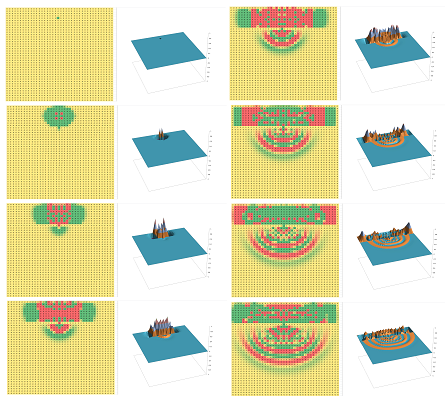
Example (breakwater). Seemingly having nothing to do with it, can our model reasonably reproduce waves of the surface of a liquid? Below we show a simulation of a breakwater protecting a harbor. It starts with a single “pulse” (tsunami?) outside the harbor, $$u(0,20,3)=1,\ u(0,x,y)=0\text{ for the rest of } (x,y),$$ and $$u(1,x,y)=0 \text{ for all } (x,y).$$ The breakwater is represented by a row of fixed values: $$u(t,x,10)=0 \text{ for all }x\ne 20,$$ with a single gap.
The large waves outside produce very mild, circular waves inside. $\square$
We repeat the algebra we used in our analysis of heat transfer for dimension $2$. When $K$ is constant, as another simplifying assumption, the total force is simplified: $$F(x_i,y_j,t_{k})=K\left( \begin{array}{ccccc} \bullet& -\Delta_yu\, (t_{k},s_{i},p_{j-1})&\bullet\\ - \Delta_x u\, (t_{k},s_{i-1},y_j)&& + \Delta_x u\, (t_{k},s_{i},y_j)\\ \bullet&+\Delta_y u\, (t_{k},s_{i},p_{j})&\bullet \end{array}\right)=K\big(\Delta_x^2 u\, (t_{k},x_{i},y_j)+\Delta_y^2 u\, (t_{k},x_{i},y_j)\big).$$ These are the second differences. Our partial difference equation becomes: $$\frac{\Delta^2 u}{\Delta t^2}=\frac{K}{m}\left(\Delta_x^2 u+\Delta_y^2 u\right),$$ where $\alpha>0$ is a constant.
Exercise. Derive a version of this equation for a variable $K$.
Just as in the $1$-dimensional case, we can argue the following two points. First, a longer spring is less stiff than a shorter one made of the same material and, therefore, $K$ is inversely proportional to $\Delta x=\Delta y$. Second, the weights are, in fact, the weights of the springs and, therefore, $m$ is proportional to $\Delta x$. Then our difference equation becomes: $$\frac{\Delta^2 u}{\Delta t^2}=\frac{\alpha}{\Delta x^2}\left(\Delta_x^2 u+\Delta_y^2 u\right)=\alpha\left(\frac{\Delta^2 u}{\Delta x^2}+\frac{\Delta^2 u}{\Delta y^2}\right).$$
Furthermore, when $u$ is defined throughout the region, the difference equation corresponds to the wave equation for partial derivatives: $$\frac{\partial^2 u}{\partial t^2}=\alpha\left(\frac{\partial^2 u}{\partial x^2}+\frac{\partial^2 u}{\partial y^2}\right),$$ with the last expression is, again, the Laplace operator of $u$.
Exercise. Derive this equation from the last.
$$\text{ THE END }$$


