This site is being phased out.
Modeling with discrete exterior calculus
Project by Julie Lang, supervised by Peter Saveliev
POSTER: Modeling Heat Transfer on Various Grids with Discrete Exterior Calculus by Julie Lang (summary)
Contents
Initial motivation
Conway's Game of Life and other cellular automata produce fascinating patterns, but, to the best of my knowledge, can't be used to model such a simple thing as a circular wave... We will be using discrete differential forms to model elementary ODEs and PDEs in dimensions 1 and 2 with C++, MATLAB, and/or Excel.
Abstract
Over the years, the heat equation has been thoroughly studied for describing how heat disperses itself through continuous media. It is well known that in a homogeneous medium, the spread of heat should be isotropic. We are interested in a discrete case, where instead of spreading heat through a single medium, the heat spreads though a grid or lattice of cells. These form a cellular complex composed of 0-cells, 1-cells, and 2-cells. In discretizing the heat equation, we base our efforts on the idea that the change in temperature of a certain 2-cell is directly proportional to the difference between its temperature and the temperature of adjacent 2-cells. In order to arrive at an equation that describes these differences while remaining as general as possible, we utilize discrete exterior calculus and differential forms. Our main conclusion is that the isotropy of heat on a grid is heavily dependant upon the geometry of the grid. For example, the square grid and the rhomboidal grid are topologically identical, but heat spreads isotropically through one and not through the other.
Newton's Law of Cooling
Those who have taken a course in partial differential equations will recognize $\frac{\partial T}{\partial t}=-k\nabla^{2} T$ as the heat equation. It is continuous and its solution relies upon both initial and boundary conditions. We are interested in a discrete version of this equation on an arbitrary grid or lattice. Essentially we want to describe how heat will distribute itself throughout an arrangement of boxes (of arbitrary shape).
To begin, we inspected a simpler idea. In a 0-dimensional continuous form, Newton's Law of Cooling is \begin{equation} \frac{d T}{d t} = -k(T-S) \end{equation} where $T$ is the temperature of some object, $S$ is the constant temperature of the object's surroundings, and $k$ is the conductivity (how easily heat can be transferred in and out of the object). In this equation, the change in temperature of the object is proportional to the difference in temperature between the object and its surroundings. The solution to this ODE is known to be \begin{equation} T = S+(T_{0}-S)e^{-kt}, \end{equation} where $T_{0}$ is the initial temperature of the object.
Square grid
However, we are interested in a discrete form of this idea. When time and space are broken up into discrete regions, the differential equation becomes \begin{equation} T_{n+1} - T_{n} = -k(T_{n}-S), \end{equation} where $T_{n}$ denotes the temperature at time step $n$. This can be extended to more dimensions. In particular, in two dimensions, the temperature of each object will depend on its temperature as well as the temperature of the four adjacent objects. In this case, the equation becomes \begin{equation} T_{n+1}^{(i,j)}-T_{n}^{(i,j)} = -\frac{k}{4} \Big[ (T_{n}^{(i,j)}-T_{n}^{(i,j-1)})+(T_{n}^{(i,j)}-T_{n}^{(i,j+1)})+(T_{n}^{(i,j)}-T_{n}^{(i-1,j)})+(T_{n}^{(i,j)}-T_{n}^{(i+1,j)})\Big], \end{equation} where $T_{n}^{(i,j)}$ denotes the temperature at time $n$ of the object in location $(i,j)$. Essentially, all we are doing is breaking it up into regions that have adjacent regions above, below, and to either side. We are then saying that the change in the temperature of our object depends on how different its temperature is from the temperature of each surrounding object, and every difference contributes equally.
Notice that the conductivity can be distributed across the difference in temperatures of nearest neighbors; it is the same for all pairs of objects. This is a homogeneous situation and it need not be the case. Suppose these objects are two-dimensional rooms, (2-cells). The conductivity would describe the thickness of the walls (1-cells) that separate the rooms. Since all walls are not necessarily the same thickness, the value of $k$ be different for each pair of adjacent rooms. This combination of "rooms" and "walls" (and "columns") is called cubical complex. This approach is different from the numerical approach to the heat equation that is presented here, but the equations are the same, initially.
We are interested in getting an equation like the one shown above in terms of differential forms. Initially, our equation was \begin{equation}\star d_{t}(T_{n}^{(i,j)})=-\frac{k}{4} \Big[ d_{x}(\star d_{x}(T_{n}^{(i-1,j)}))+d_{y}(\star d_{y}(T_{n}^{(i,j-1)})) \Big]\end{equation} where $d_{x}$ denotes an exterior derivative with respect to $x$ and $\star$ denotes the use of the Hodge Duality. Observe that the equation given above is still specific to the cubical complex. Each 2-cell has exactly four neighbors, two neighbors in the $x$ direction and two neighbors in the $y$ direction. That is why the right side of the equation begins with $-\frac{k}{4}$. To obtain a more general formula, it was proposed that one must multiply the difference between the temperatures of each pair of neighbors by a normalized number proportional to the length of the 1-cell. This equation would become \begin{equation}\star d_{t}(T_{n}^{(i,j)})=-\frac{k|\sigma|}{|\partial \alpha|} \Big[ d_{x}(\star d_{x}(T_{n}^{(i-1,j)}))+d_{y}(\star d_{y}(T_{n}^{(i,j-1)})) \Big]\end{equation} Here, $| \sigma |$ denotes the length of the 1-cell and $|\partial \alpha|$ is the length of the boundary of the 2-cell. For example, on a regular lattice, $| \sigma |$ is the length of one edge (usually kept at $1$ for convenience), and $|\partial \alpha|$ would be the perimeter of the polygon. This proposition is currently being explored and remains under revision.
We have created a program in Maple that will model heat transfer according to these rules. Our interest is in determining if this particular discretization of the heat equation is isotropic (the same in all directions). In order to do this, we are looking at a large, homogeneous two-dimensional cubical and simplicial complexes with initial conditions in which all cells are the same temperature except for one cell in the center. As time progresses, the heat will diffuse out from the center cell. If this form is indeed isotropic, a level curve should be approximately a circle. We explore level curves at half the maximum value, one fourth of the maximum value, and at arbitrarily chosen constant values.
It turns out that determining the roundness of a shape that is pixelated like this is rather difficult. It is obvious that simply looking at the image, one may determine how circular the object is, but getting a computer to look at a shape and distinguish between a circle and a square is another problem entirely. A discussion of these difficulties can be found at Roundness. In our case, we have the luxury of knowing where the center of the shape is. Currently, we are using a qualitative approach and observing plots of the level curves.
Excel
Originally, a spreadsheet was developed using Excel to investigate the aforementioned discrete heat equation. Initial conditions are set for the temperatures of the 2-cells and then these are allowed to change according to the following equation. Using the R1C1 reference style, (that is found under Excel options / Formulas; it refers to a cell by its row and column) the formula for a cell that is not on a boarder is
=(R[-1]C*(R[-2]C-RC)+R[1]C*(R[2]C-RC)+RC[-1]*(RC[-2]-RC)+RC[1]*(RC[2]-RC))/4+RC.
Each cell would successfully refer to adjacent cells and had been modified to include different boundary conditions such as each 2-cell on a boarder simply having a reduced number of neighboring cells. Other boundary conditions have connected one side to another in a variety of ways. These modifications change the topology of this lattice to be a cylinder, a torus, a Mobius strip, and a Klein bottle. However, Excel did not iterate in the particular way that was needed. In order for a program to be successful, when an iteration occurs, the new value in each cell depends only the previous values of that cell and its neighboring cells. When the Excel sheet performed an iteration, it would evaluate cells sequentially. So the new value of a cell would be calculated from the previous values of some adjacent cells and the new values of other adjacent cells.
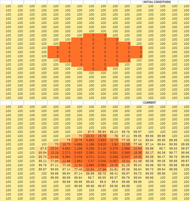
This is shown at t=1. Since just a single iteration has been carried out, only the cells that were on the edge of the cold spot in the center should have changed temperature. However, this is not the result that Excel produces. (One can deal with this by using an extra sheet as a buffer but this didn't seem worth the effort...)
Maple
Therefore, this approach was set aside and a new program was written using Maple. This designates the 2-cells as elements of an $n \times m$ matrix. Originally, the conductivities $k$ were held in an $n \times 2m$ matrix. Twice as many elements were needed for this matrix because it must not only contain conductivities for vertically adjacent cells, but also horizontally adjacent cells. But our focus is more on a homogeneous case, so for the purposes of speed of the program,the conductivity matrix was replaced with a constant $k=0.6$.
As has been mentioned, the initial conditions begin all cells at $T_{0}=0$ except for the center cell, for which $T^{center}_{0}=10000$. The current version of the program models a $250 \times 250$ complex in a homogeneous medium with $k=0.6$. We try to keep the lattice large to decrease edge effects as the heat disperses. Boundary conditions are that each cell on the boarder simply has a smaller number of adjacent cells. For example, $T^{0,0}$ only depends on $T^{0,1}$ and $T^{1,0}$. It should be noted that these boundary conditions are not essential; our program is terminated before the cells on the boarder can noticeably change.
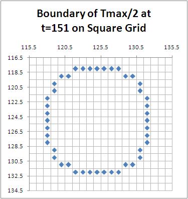
We are interested in determining if this model is isotropic. In order to do this, we take level curves of this matrix at varying times and observe the shape of these curves. We began by taking a level curve at $T_{max}/2$. In order to determine its shape, the program records the row and column of all cells with values of $T$ that are greater than $T_{max}/2$ and are adjacent to cells with values of $T$ that are less than $T_{max}/2$. These coordinates are then copied to an Excel sheet where they are plotted. For example,
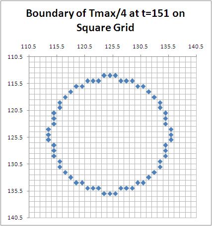
One can see that this shape could be seen as circular, but it could be taking on the shape of an octagon. Due to the relatively small radius, whether or not this is approaching a circle or an octagon is unclear. Therefore, we also investigated the level curve at $T_{max}/4$. Looking at a lower value should increase the size of our shape and show a less ambiguous figure.
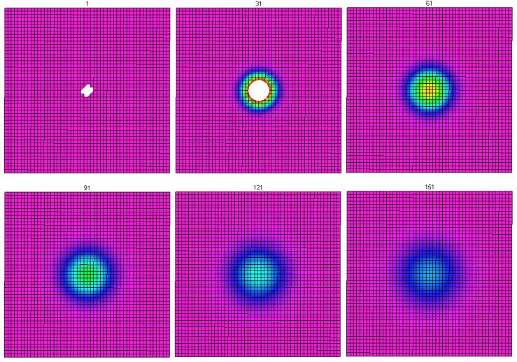
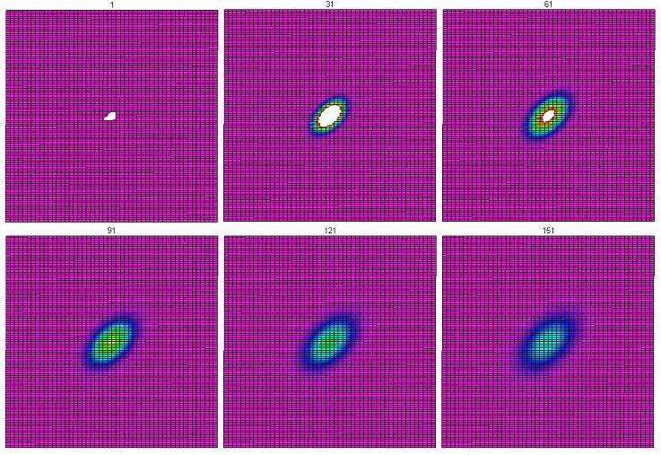
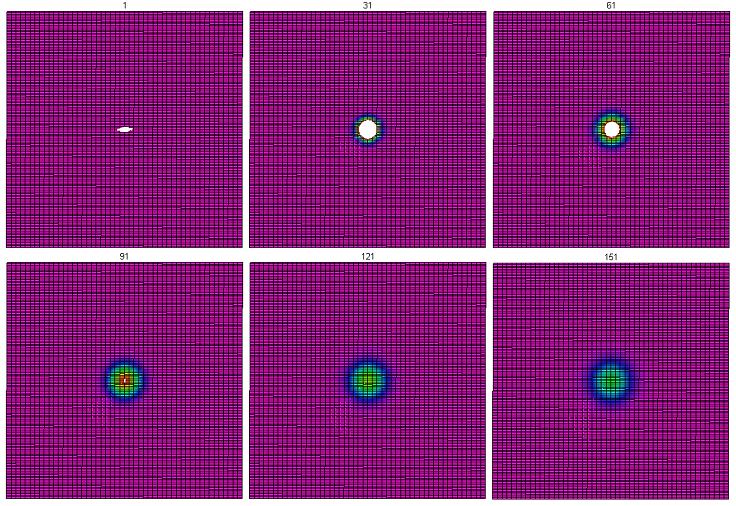
Plotting the edges of these level curves was very inefficient and tedious. Once we were able to utilize Maple's plotting features, we are able to get a clearer idea of how this is evolving. This is the middle $50 \times 50$ portion of the grid (we did not include the outer part in these pictures since the temperature in those cells does not change noticeably before the program terminates). Color indicates temperature on a ROYGBV spectrum, where red indicates higher temperatures and purple indicates lower temperatures. White is hotter than red. The time is given on the top part of each picture.
From this, it appears as though the heat is spreading uniformly in all directions.
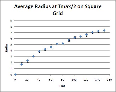
To investigate whether or not this shape is indeed a circle, we look at the distance of each of these cells from the origin of the heat (the center cell that began with $T=10000$). So using the distance formula, an average radius can be determined. This does change over time, so here is a graph of that evolution for the level curve at $T_{max}/2$.
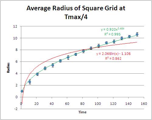
Notice the small standard deviations. One would expect that as the radius grows, the standard deviation would shrink. That is, if the shape is approaching a circle, the spread of the distances of the center would diminish. It would also make sense that the graph would have the same shape for all level curves. So here we have a graph of the level curve at $T_{max}/4)$.
One can see that these graphs are very similar. It was noted that these look like they may follow a logarithmic or square root. Excel was used to fit this graph with the trend-lines that are shown. A logarithmic fit is in red and a power fit is in green. The value of $R^{2}$ for the power is 0.995 and the exponent is 0.484. This is expected, since it is known that heat diffuses through a homogeneous media like a square root.
Triangular grid
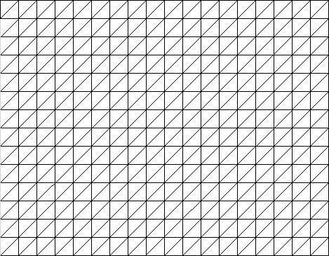
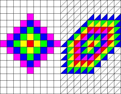
We were interested in whether we would find the same results on a different grid. We are looking at a triangular grid such as the one pictured below.
The reason we are using this grid instead of one composed of equilateral triangles is simply for convenience. Since a program already existed for a regular square lattice, one need only modify the formula for the neighboring 2-cells to achieve a lattice like this. In addition, this grid So we used an analogous formula for the triangular grid: \begin{equation} T^{i,j}_{n+1}=-\frac{k}{3} \Big[ (T^{i+1,j}_{n}-T^{i,j}_{n})+(T^{i-1,j}_{n}-T^{i,j}_{n})+(T^{i+(-1)^{i+1},j+(-1)^{i}}_{n}) \Big]+T^{i,j}_{n}\end{equation} Preliminary results are shown below.
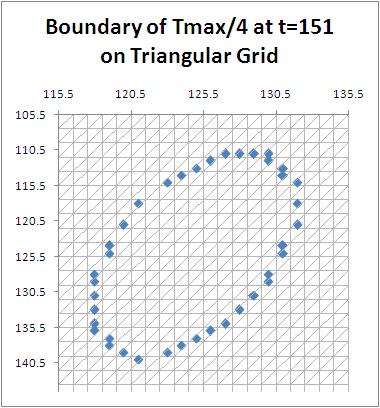
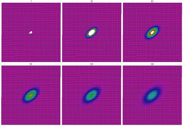
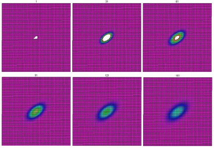
The boundary of the level curve at $T_{max}/4$ is shown above. The axes have been modified so that it resembles the first lattice shown. Here is another image as the temperature distributes itself across the grid (again, on the ROYGBV spectrum, just as it is above). However, instead of showing the middle $50 \times 50$ portion, this shows the center $100 \times 50$ portion, so that it will maintain the same shape as the two figures above.
This shape appears to be non-circular. This is most likely due to the structure of the grid. However, one must keep in mind that the length of each side has not been taken into account in this run; all 1-cells are treated as if they are of the same length.
It was suggested that this shape looked like a hexagon that was made from expanding through to neighboring triangular cells, similar to a diamond shape that is made from expanding to neighboring cells of a square lattice.
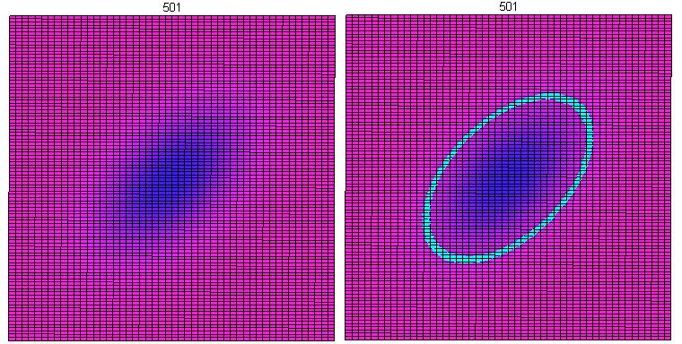
Since after a short time, the diffusion of heat on the square lattice overcomes the diamond shape, it is not unreasonable to think that the triangular lattice would do the same after a long period of time. However, that is not the case. As seen below, at t=501, the shape is still oblong. (The second copy of this has highlighted the cells with temperatures between 4 and 5, just for clarity).
Another proposed solution was that we should begin with two 2-cells at 10000, not just one. The idea was that having only one cell with a high temperature made it much more likely for the heat to spread in the direction of the neighbors of the original center cell. So, say that the center cell has neighboring cells above and below it, but also one diagonally up and to the right. Since there is not a neighboring cell down and to the left, it was thought that this could be giving the heat dispersion a preferred direction. In order to test this idea, we began with all cells at $T=0$, except for the center cell and one of its neighbors, which are at $T=10000$. This neighbor was chosen so that it, along with the center cell, would form a square. This would eliminate any bias due to the configuration of adjacent cells at $t=0$.
One can see that beginning with two cells at $T=10000$ still produces the oblong shape. This means that the initial conditions are not affecting the directions in which the heat disperses.
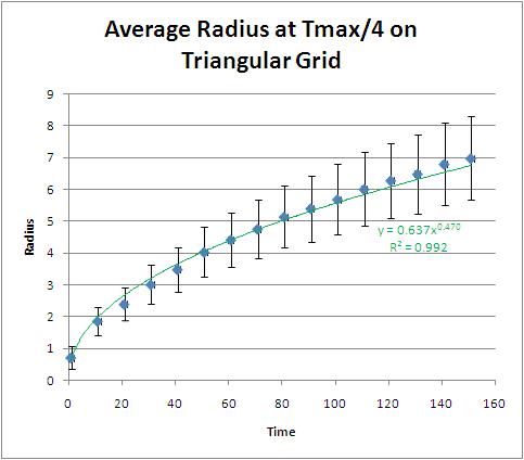
Here is a plot of the average radius of these shapes as it changes with time. Notice that the standard deviations are increasing with time! That suggests that the shape is not a circle.
We also plan on changing the meaning of "radius" to be "number of 2-cells away from the center". That is to say that we would use a taxicab metric for the square lattice and employ a similar metric for the triangular lattice.
A modification was proposed as an attempt to make this equation isotropic for an arbitrary lattice. In this model, the conductivity is multiplied by $\frac{|\sigma|}{|\partial\alpha|}$. That is, the ratio of the length of the wall (1-cell) to the perimeter of the room (2-cell). The idea behind this modification was to make more heat go through the longer 1-cells. Clearly, if one were to construct a physical room in which one wall was longer than all the others, more heat would go through that wall overall. This would leave the equation for the square lattice unchanged (since each edge is 1/4 the perimeter), but it would have an effect on the triangular grid. The legs of each triangle are defined to have length 1, then the hypotenuse has length $\sqrt{2}$. The boundary of the 2-cell has length $\sqrt{2}+2$. Therefore, the equation becomes \begin{equation} T^{i,j}_{n+1}=-\frac{k}{\sqrt{2}+2} \Big[ (T^{i+1,j}_{n}-T^{i,j}_{n})+(T^{i-1,j}_{n}-T^{i,j}_{n})+\sqrt{2}(T^{i+(-1)^{i+1},j+(-1)^{i}}_{n}) \Big]+T^{i,j}_{n}.\end{equation} However, this approach does not yield the desired results.
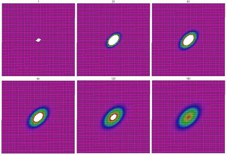
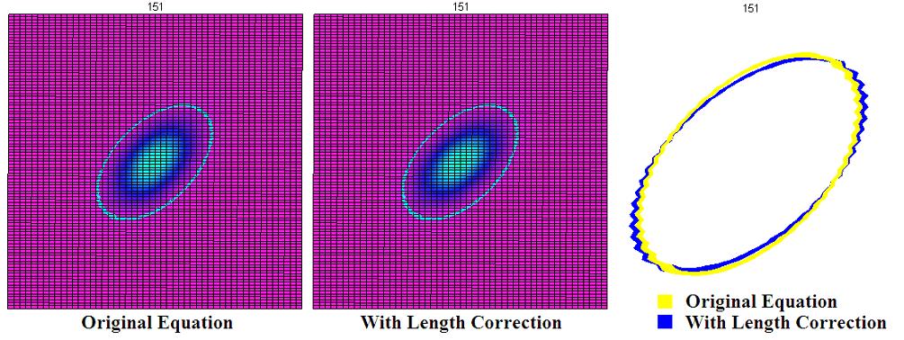
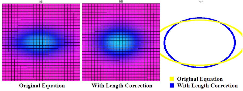
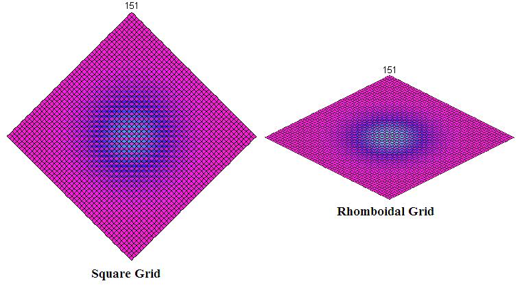
Unfortunately, we still see the stretched shape! Comparing the results of the original equation to those of the equation with the length correction, we do see that there is a difference. Below, plots of the center portion of both equations at $t=151$ are shown side by side, with the cells with temperatures between 4 and 5 highlighted. On the far right, we compare the shapes of these curves. The equation with the length correction is more stretched than the original equation!
Further analysis is in progress. We hope to find some other modification to create an isotropic equation on an arbitrary lattice. Nonetheless, we will further explore the oddities presented in the triangular lattice.
Rectangular grid
Due to the complexities brought about by the triangular lattice, it was proposed that we should investigate a rectangular lattice. It would be quite similar to the square lattice in that each 2-cell would have 4 adjacent 2-cells and the 2-cells would be lined up in rows and columns that are at 90 degrees to each other. But it would be similar to the triangular lattice in that the 2-cells are not regular; some sides are longer than others. Therefore, using the length corrected formula for a $2 \times 1$ rectangle, (that is, $\star d_{t}(T_{n}^{(i,j)})=-\frac{k|\sigma|}{|\partial \alpha|} \Big[ d_{x}(\star d_{x}(T_{n}^{(i-1,j)}))+d_{y}(\star d_{y}(T_{n}^{(i,j-1)})) \Big]$) we arrived at this equation: \begin{equation} T_{n+1}^{(i,j)}-T_{n}^{(i,j)} = -\frac{k}{6} \Big[ (T_{n}^{(i,j)}-T_{n}^{(i,j-1)})+(T_{n}^{(i,j)}-T_{n}^{(i,j+1)})+2(T_{n}^{(i,j)}-T_{n}^{(i-1,j)})+2(T_{n}^{(i,j)}-T_{n}^{(i+1,j)})\Big] \end{equation} Modifying the Maple program to run according to this rule, our results follow.
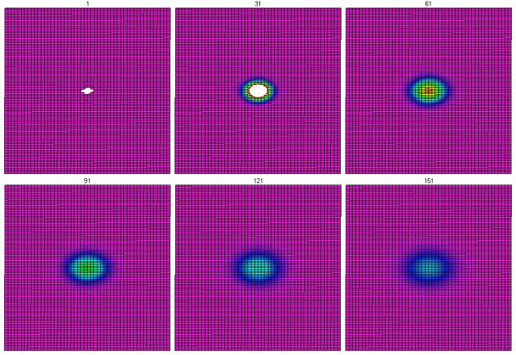
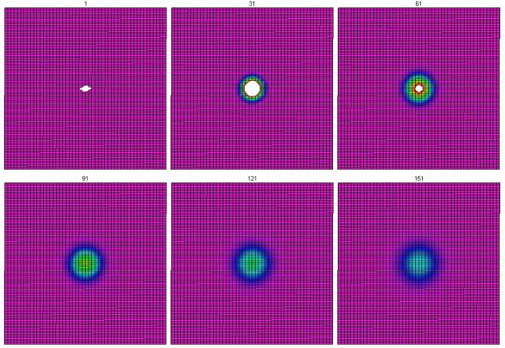
Curiously, this does not form a circle like one would have expected! So one thing is undeniably clear: the structure of the grid has more of an affect on the diffusion of heat than we originally considered.
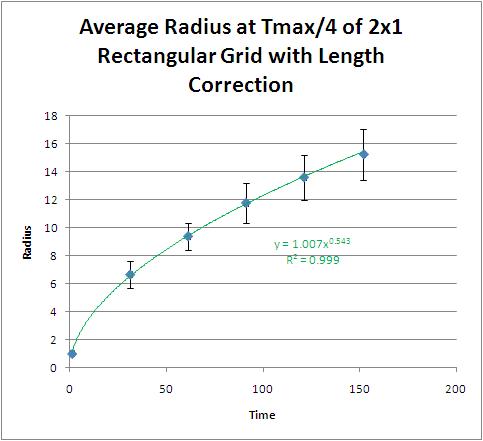
Here is a plot of the average radius as it changes with time. Note that it still follows a square root, but the standard deviations increase with the number of iterations. This indicates that the shape is not circular.
However, the correction for the different lengths of the 1-cells has greatly improved the roundness of this shape. It is not quite a circle, but when compared with the equation that did not take into account the different values of $|\sigma|$, is has become much more circle-like!
Therefore, the length correction has improved our model. We simply need to add more adjustments. These modifications are discussed below.
Our hopes are to arrive at an equation that will work on an arbitrary mesh. Our next idea was to not only consider the lengths of the 1-cells, but also to consider the lengths of the 1-cells in the dual grid. (The dual grid is the grid formed from replacing 2-cells with 0-cells, changing the orientation of 1-cells, and replacing 0-cells with 2-cells. For a cubical complex, the dual grid is another cubical complex that has been translated. For a hexagonal complex, it is another hexagonal complex. For a triangular complex, however, the dual grid is a hexagonal complex.) By incorporating the length of the 1-cells of the dual grid, we are computing the distance between the centroid (the "center of mass") of our 2-cells. This changes under the same transformations that (for example) turn a square grid into a rectangular grid.
It is clear from the information and evidence above that the 2-cells that have a smaller 1-cell between them on the dual grid (that is, the 2-cells with closer centers of mass) should exchange more heat than those with a larger 1-cell on the dual grid. (For simplifying the terminology, I will refer to this 1-cell as the 1*-cell.) Therefore, we consider including the quantity $1/|\sigma^{*}|$ into our formula. This quantity will be larger for smaller 1*-cells. But we must remember to normalize it! Therefore, we used the following modification to the formula. In addition to multiplying each difference in temperatures of adjacent 2-cells by $|\sigma|$, we also wish to divide it by $|\sigma^{*}$. That is, we are multiplying by the ratio between the length of a 1-cell and the length of its dual. This quantity must then be normalized, resulting in the equation \begin{equation} d_{t}T(\alpha)^{*} = \Big[ \int_{\partial \alpha} \frac{|a|}{|a^*|} \Big]^{-1} \int_{\partial \alpha} k(a)(d_{x}T^{*})(a^{*}) \frac{|a|}{|a^{*}|} \end{equation} Here, $\alpha$ is a 2-cell and $a$ is a 1-cell on its boundary. Notice that these modifications leave the equation of for the square grid unchanged, but it changes for the other grids.
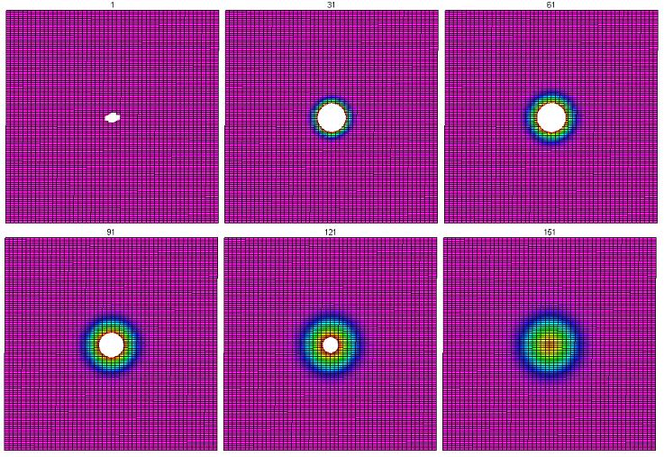
When this was implemented for the $2\times 1$ rectangular lattice, the result was circular.
To check to make sure that the initial shape of the signal is not responsible for the circular shape, the same equation was run on the $2 \times 1$ rectangular grid, but beginning with two central rectangles with temperature of 10000. The two rectangles together form a square, the same initial shape that we have in the other cases. The results are also circular.
This correction to our equation was also sufficient to result in a circle for a $3 \times 1$ grid.
Compare this with the evolution of the $2 \times 1$ rectangular grid. The heat is traveling through the medium at a much slower rate in the $3 \times 1$ case! Unfortunately, due to time constraints, we are unable to explore this in depth. Yet the results from the $2 \times 1$ and the $3 \times 1$ rectangular grids suggests that this formula will be isotropic for any rectangular grid.
However, our correction did not result in a circle for the triangular lattice.
The following is the Maple code for the 3x1 rectangular grid. This would probably be more appealing if it were a link to a different page, but I am uncertain as to how to make that happen.
with(plots):
with(LinearAlgebra):
interface(rtablesize = 10000):
interface(displayprecision):
Digits := 3:
rows := 250:
columns := 250:
iter := 151: #iter is the maximum of t
bound := 1: #This is old. If I get time, I will take it out.
centi := floor((rows+1)*(1/2)):
centj := floor((columns+1)*(1/2)):
initfunc := (i, j) -> piecewise(i = centi and j = centj, 10000, 0.1e-3): #This determines the initial conditions -- everything is 0.0001 except for the center cell
Initial := Matrix(rows, columns, initfunc):
klong := .6*(3/(6.666666666)): #these are a conductivity of .6 multiplied by the length of a 1-cell, divided by the
                               sum of the ratio of the length of the 1-cells to the length of their duals
kshort := .6*(.3333333333/(6.666666666)):
Prev := Initial:
for t to iter do
   if bound = 1 then
      f := (i, j) -> piecewise(i != 1 and i != rows and j != 1 and j != columns,
           klong*(Prev(i-1, j)-Prev(i, j))+klong*(Prev(i+1, j)-Prev(i, j))+kshort*(Prev(i, j-1)-Prev(i, j))+kshort*(Prev(i, j+1)-Prev(i, j))+Prev(i, j),
           i = 1 and j != 1 and j != columns,
           (klong*(Prev(i+1, j)-Prev(i, j))+kshort*(Prev(i, j-1)-Prev(i, j))+kshort*(Prev(i, j+1)-Prev(i, j)))*(1/5)*6.666666666+Prev(i, j),
           i = rows and j != 1 and j != columns,
           (klong*(Prev(i-1, j)-Prev(i, j))+kshort*(Prev(i, j-1)-Prev(i, j))+kshort*(Prev(i, j+1)-Prev(i, j)))*(1/5)*6.666666666+Prev(i, j),
           j = 1 and i != 1 and i != rows,
           (klong*(Prev(i-1, j)-Prev(i, j))+klong*(Prev(i+1, j)-Prev(i, j))+kshort*(Prev(i, j+1)-Prev(i, j)))*(1/7)*6.666666666+Prev(i, j),
           j = columns and i != 1 and i != rows,
           (klong*(Prev(i-1, j)-Prev(i, j))+klong*(Prev(i+1, j)-Prev(i, j))+kshort*(Prev(i, j-1)-Prev(i, j)))*(1/7)*6.666666666+Prev(i, j),
           i = 1 and j = 1,
           (klong*(Prev(i+1, j)-Prev(i, j))+kshort*(Prev(i, j+1)-Prev(i, j)))*(1/4)*6.666666666+Prev(i, j),
           i = rows and j = 1,
           (klong*(Prev(i-1, j)-Prev(i, j))+kshort*(Prev(i, j+1)-Prev(i, j)))*(1/4)*6.666666666+Prev(i, j),
           i = 1 and j = columns,
           (klong*(Prev(i+1, j)-Prev(i, j))+kshort*(Prev(i, j-1)-Prev(i, j)))*(1/4)*6.666666666+Prev(i, j),
           i = rows and j = columns,
           (klong*(Prev(i-1, j)-Prev(i, j))+kshort*(Prev(i, j-1)-Prev(i, j)))*(1/4)*6.666666666+Prev(i, j),
           Prev(i, j): #Note: the "not equal to" is denoted "!="
                              and that the structure of piecewise functions in Maple is piecewise([condition],[formula],[condition],[formula],else).
                              Spaces have been added for ease of reading. In Maple, it must be evaluated as one line of code.
      current := Matrix(rows, columns, f):
      Prev := current:
      if `mod`(t, 30) = 1 then
         a := .25*max(current): print(t); boarderi := []: boarderj := []: dist := []:
         #Prints time, and the x,y coordinate of a point on the boarder of a level curve, along with its distance from the center.
         for i from 2 to rows-1 do
            for j from 2 to columns-1 do
               if current(i, j) > a then
                 if `or`(`or`(`or`(current(i+1, j) < a, current(i-1, j) < a), current(i, j+1) < a), current(i, j-1) < a) then
                    d := sqrt((centi-i)^2+(2*(centj-j))^2):
                    boarderi := [op(boarderi), i]:
                    boarderj := [op(boarderj), j]:
                    dist := [op(dist), d]:
                 end if:
              end if:
           end do:
        end do:
        print(boarderi);
        print(boarderj);
        print(dist);
        if `mod`(t, 30) = 1 then
           print(t);
           print(matrixplot(current, orientation = [0, 0], shading = zhue, view = [50 .. 200, 100 .. 150, 0 .. 100], title = t));
           print();
        end if:
        if t = 151 then
           print(t);
           print(matrixplot(current, orientation = [0, 0], shading = zhue, view = [88 .. 162, 113 .. 138, 0 .. 100], title = t));
        end if:
     end if:
  end if:
end do:
I'll finish cleaning this up after class, I promise.
Rhomboidal grid
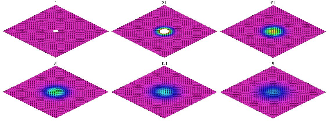
It has been suggested that this modification fails on the triangular grid due to the structure of the grid being "slanted". We are in the process of trying to quantify this "slantedness" and include that in our equation. However, in order to look at this idea in a more simple case, we are examining a rhomboidal grid. This will be exactly like the square grid with the exception of a difference in angles. The ratio of the length of the 1-cells to the lengths of their duals will always be 1, so both of the adjustments that have been made are moot. Therefore, running this formula will produce results like those that follow.
Notice that the simple act of adjusting the angles of the 2-cells on our grid has drastically distorted the global properties of our heat distribution! Therefore, we have attempted to find some way to compensate for this change. Since the lengths of all 1-cells (and their duals) are equal to 1, we must concern ourselves only with the orientation of the 1-cells and the 1*-cells. We have made efforts to define this solely in terms of local properties. After a good deal of inspection, our first approach had to do with comparing one cell to its "second degree neighbors". That is, the neighbors of the neighboring cells. For example, in [1], the second degree neighbors of the central red cells would be the green cells. The reason for this approach was because although the lengths of the 1-cells are exactly the same, the distances between the centroid of the center cell and the centroid of a second degree neighbor varies with changes in the angles. In addition, it does not seem unreasonable to incorporate the locations of three 2-cells (the center 2-cell, the first degree neighbor of the center cell, and the second degree neighbor of the center cell). Since the original heat equation, $\frac{\partial T}{\partial t} = -k \nabla^{2}T $, involves a second spacial derivative, using the positions of three cells would be similar. It turns out that in the homogeneous case on a rhomboidal grid, all dependence on the first degree neighbors cancels out. Therefore, our model only considers every other cell! We implemented a formula that considers the difference between the temperatures of second degree neighbors and the ratio of the length of the two 1-cells to the length of the chain that consists of two 1*-cells.
We began with a square grid. Since this revision only utilizes every other cell, it is helpful to have a control to which we may compare the rhomboidal grid.
It is clear that even though the distances between the centroids of the 2-cells does vary, it is not enough to compensate for the preferential direction brought about by the slantedness of the grid.
Background
- Prerequisite: Linear algebra: course and Differential equations: course, some computer language
- Co-requisite: Differential forms: course
We aren't really after differential equations, i.e., equations with respect to derivatives, but rather equations with respect to differential forms. If you look at the derivations of these equations, you can make a switch...
Further research
- fluid flow from a vector field
- wave equation
