Linear functions in Euclidean space

Linearity

First let's address some terminology...

$f(x) = 2x + 3$ is NOT a linear function!

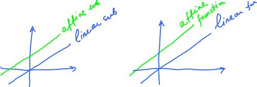
Why??? We are used to this terminology in calculus. But here it is the $3$ that makes it non-linear. Such a function is called "affine" or you can call it a linear polynomial. This makes sense in light of what we mean by linear and affine subspaces. Below we have linear and affine subspaces on the left and then, on the right, they are interpreted as the graphs of two functions.

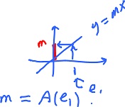
The example suggests that $f \colon {\bf R} \rightarrow {\bf R}$ is a linear function only if has the form: $$f(x) = mx.$$

In other words, here each $x$ is multiplied by the same number. That's a linear procedure! But $mx+b$ is not.

Let's look at the properties of a function of this kind.

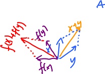
Addition is preserved under $f$:

If $f(x) = X$ and $f(y) = Y$, then $f(x + y) = X + Y$.

Here $x + y$ is the input and $X + Y$ is the output of $f$.

Let's instead consider $$f(x) = 3x + 1,$$ then $$f(x + y) = 3(x + y) = 3x + 3y + 1;$$ $$f(x) + f(y) = 3x + 1 + 3y + 1 = 3x + 3y + 2.$$ These functions are not equal! Thus $3x+1$ does not preserve addition, so it’s not linear.

Scalar multiplication is preserved under $f$:

If $f(x) = X$, then $f({\alpha}x) = {\alpha}X$.

Instead consider $$f(x) = 3x + 1,$$ then $$f(2x) = 3(2x) + 1 = 6x + 1;$$ $$2f(x) = 2(3x + 1) = 6x + 2.$$ These functions are not equal!

There is another connection to linear algebra. The set $$\{f_m(x) = mx \colon m \in {\bf R} \}$$ is the collection of all linear functions ${\bf R} \rightarrow {\bf R}$. Now, every function from this collection is represented as a product. Similarly we can consider the set of all products $$f_m(x) = <m,x>$$ as the set of linear functions $$f_m \colon {\bf R}^2 \rightarrow {\bf R}.$$ Indeed the linearity follows from the formula of the inner product:

if $x = (x_1,x_2), m = (m_1,m_2)$ then $<m,x> = m_1x_1 + m_2x_2.$

More generally the linearity of $$f_m = <m,\cdot> \colon {\bf R}^n \rightarrow {\bf R}$$ follows from the properties of the inner product. Indeed,

• Distributivity Property => addition is preserved,
• Homogeneity Property => scalar multiplication is preserved.

Now, what is linearity?

A linear function preserves vector operations:

• scalar multiplication: $f(ax) = ax$, and
• addition: $f(x + y) = f(x) + f(y)$.

Example. Consider $$f(x) = 3x + 1.$$ Addition is preserved if under $f$:

$x \mapsto X$ and $y \mapsto Y \mapsto x + y \mapsto X + Y$

But: $$f(x + y) = 3(x + y) + 1 = 3x + 3y + 1$$

$f(x) + f(y) = 3x + 1 + 3y + 1 = 3x + 3y + 2$ (the functions are not equal)

Thus, $3x + 1$ does not preserve addition, so it is not linear.

Scalar multiplication is preserved if under $f$: $$x \mapsto X \mapsto {\alpha}x \mapsto {\alpha}X.$$ But: $$f(2x) = 3(2x) + 1 = 6x + 1,$$

$2f(x) = 2(3x + 1) = 6x + 2$ (the functions are not equal).

Again, $y = 3x + 5$ is a "linear function" in any calculus course, not in Advanced Calculus ...

• f(x) = 3x + 5 - linear?
• f(x) = 3x - linear!

(The functions have same derivative though.)

Let's preview how we'll use linear function in calculus.

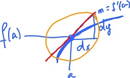
Dimension 1. Consider $$y = f(x) at x = a.$$ Then

$f’(a)$ is a number.

Further

$dy/dx = f’(a)$ and $dy = f’(a)dx$ is linear function of $dx$ (multiplication by a constant number)

Dimensions $2$ (and $3$, $4$, $5$...). Consider

$f \colon {\bf R}^2 \rightarrow {\bf R}$, given by $dy = <f’(a),dx>$, where $m = (\frac{\partial f}{\partial x}, \frac{\partial f}{\partial y}) = f’(a)$ is the gradient.

Once again this is a linear function.

Vector functions. What if we have a vector function $$f: {\bf R}^n \rightarrow {\bf R}^m?$$ Then we have a similar representation of its derivative (the Jacobian):

$dy = f’(a)(dx)$, where $f’(a)$ is a matrix.

This is a linear function.

These examples explain why we need linear functions in calculus.

Now let's inject some geometry into this. Recall

$A \colon {\bf R}^n \rightarrow {\bf R}^m$ is a linear function if it preserves the vector operations.

For example,

$n = m = 2 \rightarrow A$ is a $2 \times 2$ matrix.

What we need here: multiply by $2$, then apply $A$, or apply $A$, then multiply by $2$, should yield the same result: $$A(2x) = 2A(x)$$

Example. (1) Suppose $A \colon {\bf R}^n \rightarrow {\bf R}^n$ is a "stretch".

Then each $x$ is multiplied by a constant, say $2$: $$A(x) = 2x.$$ Then $A$ is linear!

(2) Suppose $A \colon {\bf R}^2 \rightarrow {\bf R}^2$ is a rotation around $0$

(what is the matrix?). It's linear!

(3) Suppose $A \colon {\bf R}^n \rightarrow {\bf R}^n$ is a "flip" ($A(x) = -x$): $$-(x + y) = -x + (-y)$$ $$-({\alpha}x) = {\alpha}(-x).$$ It's linear!

(4) Suppose

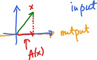
• $A: {\bf R}^2 \rightarrow {\bf R}$ is the projection:
• $A(x,y) = x$.

Also linear.

Example. Suppose $A(x_1, x_2) = (2x_1 - x_2, x_1 + 3x_2).$ Then $$\begin{array}{} A({\alpha}x_1, {\alpha}x_2) &= [2({\alpha}x_1)-({\alpha}x_2), ({\alpha}x_1) + 3({\alpha}x_2)] \\ &= {\alpha}(2x_1 - x_2, x_1 + 3x_2) \\ &= {\alpha}A(x_1, x_2); \end{array}$$

$$\begin{array}{} A(x_1 + y_1, x_2 + y_2) &= {\rm \hspace{3pt} ..some \hspace{3pt} simple \hspace{3pt} algebra...} \\ &= A(x_1, x_2) + A(y_1, y_2) \end{array}$$

See also Affine functions.

Definition and properties

Definition. A function $A \colon S \rightarrow T$, where $S, T$ are linear spaces, is a linear function if:

1. $A(x + y) = A(x) + A(y)$ for all $x,y \in S$;
2. $A({\alpha}x) = {\alpha}A(x)$ for all $x \in S, {\alpha}\in{\bf R}$.

Properties. Suppose $A$ is linear, then

1. $A(0) = 0$ (indeed $A(0 \cdot x) = 0 \cdot A(x) = 0)$;
2. $A(-x) = -A(x)$;
3. $A({\alpha}x + \beta y) = {\alpha}A(x) + \beta A(y)$ (to prove apply (1) and (2) consecutively).

Example. A linear scalar function can be represented as inner product. But also the inner product is a linear function:

$A \colon {\bf R}^2 \rightarrow {\bf R}$ given by $A(X_1, X_2) = <(a,e), (X_1,X_2)>.$

For example $$A(X_1, X_2) = 3X_1 - 5X_2 = <(3,-5), (X_1,X_2)>.$$

Example. What about the norm? Consider

$$|| \cdot || \colon {\bf R}^2 \rightarrow {\bf R}.$$

Then,

• $||{\alpha}X|| = |{\alpha}| \cdot ||X||$ Homogeneity Property.

But here $|{\alpha}|$ is a positive value! Indeed

$$||-X|| = ||X|| {\rm \hspace{3pt} not \hspace{3pt}} -||X||.$$

Also

$$||X + Y|| \leq ||X|| + ||Y|| {\rm \hspace{3pt} not \hspace{3pt}} =.$$

So, $||X||$ is not linear.

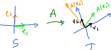
Next, what if we choose $x = e_1, y = e_2$ (the basis vectors)?

$$A({\alpha}e_1 + \beta e_2) = {\alpha}A(e_1) + \beta A(e_2);$$

First observe that since every vector can be represented as a linear combination of the basis vectors, $A$ is essentially a function of ${\alpha}, \beta$. Also the right hand side is also a linear combination of basis vectors. Then, to compute $A(X)$, where $X = ({\alpha}, \beta )$, all you need is to find $A(e_1), A(e_2)$. (The idea is illustrated in the $1$-dimensional case on the right.)

Need the basis vectors for $T={\bf R}^2$.

$$A \colon S \rightarrow T, S = {\bf R}^2, T = {\bf R}^2.$$

Always for each $x$, there are $a,b$ such that

$$A(x) = av_1 + bv_2.$$

So, let's express the output of $A$ in terms of the basis of $T, v_1, v_2$, specifically

$A(e_1) =$ linear combination of $v_1, v_2$;
$A(e_2) =$ ....

How? $$A(e_1) = a_{11}v_1 + a_{12}v_2;$$

$$A(e_2) = a_{21}v_1 + a_{22}v_2;$$

Since $v_1, v_2$ are always repeated for all $x$, we only collect the coefficients:

$$\rightarrow |a_{11} a_{12}|;$$

$$|a_{21} a_{22}|;$$

This is called a matrix of $A$.

Matrix representation of linear functions

Example.Suppose $$A(x_1, x_2) = (2x_1-x_2, x_1+5x_2)$$

Find the coefficients of the matrix: $a_{11}...a_{22}$.

Here $x_1, x_2$ are the coordinates of $X = (x_1, x_2)$ with respect to $e_1, e_2$, the basis. Now

$A(e_1) = A(1,0) = (2,1) \longleftarrow$ representations
$A(e_2) = A(0,1) = (-1,5) \longleftarrow$ with respect to $v_1, v_2$.

In other words,

$$A(e_1) = 2v_1 + v_2;$$

$$A(e_2) = -v_1 + 5v_2.$$

Then $$a_{11} = 2, a_{12} = -1;$$

$$a_{21} = 1, a_{22} = 5.$$

Using the matrix notation: $$A(x_1, x_2) = \left| \begin{array}{} 2 & -1 \\ 1 & 5 \end{array} \right| \left| \begin{array}{} x_1 \\ x_2 \end{array} \right| = (2 \cdot x_1 - 1 \cdot x_2, 1 \cdot x_1 + 5 \cdot x_2).$$

Or:

$$A(x_1, x_2) = (2x_1 - x_2, x_1 + 5x_2).$$

We represented $A$ as a matrix, then the function is recovered by computing the matrix product $AX$ for $X \in {\bf R}^2$.

More generally,

$A \colon {\bf R}^n \rightarrow {\bf R}^m$ is a matrix $m \times n$ ($m$ is # of rows and $n$ is # of columns).

$$\left| \begin{array}{} a_{11} & a_{12} & \ldots & a_{1n} \\ a_{21} & a_{22} & \ldots & a_{2n} \\ \vdots \\ a_{m1} & a_{m2} & \ldots & a_{mn} \end{array} \right| \left| \begin{array}{} x_1 \\ x_2 \\ \vdots \\ x_n \end{array} \right| = \left| \begin{array}{} a_{11}x_1 &+ a_{12}x_2 &+ \ldots &+ a_{1n}x_n \\ a_{21}x_1 &+ a_{22}x_2 &+ \ldots &+ a_{2n}x_n \\ \vdots \\ a_{m1}x_1 &+ a_{m2}x_2 &+ \ldots &+ a_{mn}x_n \end{array} \right|$$

Or

$( m \times n$ matrix $) ( n$-vector $) = ( m$-vector ).

In the left hand side $n$ and $n$ match.

Let's consider linear functions from ${\bf R}^n$ to ${\bf R}^m$.

Example. Suppose

$A \colon {\bf R}^2 \rightarrow {\bf R}^2$ is the stretch by $2$.

Then $$A = \left| \begin{array}{} 2 & 0 \\ 0 & 2 \end{array} \right|$$

Subspaces associated with a linear function

What is the "range" of a linear function? Recall the definition from Calculus:

Range of $f = \{y \colon f(x) = y$ for some $x \}.$

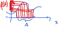
Given a function $f \colon {\bf R}^n \rightarrow {\bf R}^m$, and a subset $A \subset {\bf R}^n$, the image of $A$ under $f$ is:

$f(A) = \{y \in {\bf R}^m \colon f(x) = y,$ for some $x \in A \}.$

This is the terminology we will use instead of "range".

Also, the image of f is $f({\bf R}^n)(=$range) or:

$${\rm Im}(f) = \{y \colon y = f(x) \}.$$

Theorem. Given $f \colon {\bf R}^n \rightarrow {\bf R}^m$ a linear function, and $A \subset {\bf R}^n$ a linear subspace, then

$f(A) \subset {\bf R}^m$ is a linear subspace.

Proof. Verify the closedness of $f(A)$ under the operations: $y_1, y_2 \in f(A)$, then $y_1 = f(x_1), y_2 = f(x_2)$. Then

$$\begin{array}{} y_1 + y_2 &= f(x_1) + f(x_2) \\ &= f(x_1 + x_2). \end{array}$$

Here $x_1 + x_2 \in A$ since $A$ is a subspace, so $f(x_1 + x_2) \in f(A)$. QED

Exercise. What about scalar multiplication?

Example. Suppose $f$ is a motion of ${\bf R}^2$ (with fixed $0$). Then

$${\rm Im}(f) = {\bf R}^2.$$

According to the theorem, the options are:

• $0$, a line, or ${\bf R}^2$.
• ${\rm Im}(f) = 0$, only one possibility $f(x) = 0$ for all $x$ is the constant function.
• ${\rm Im}(f) =$ a line, for example $f(x_1, x_2) = (x_1, 0)$ is the projection.
• ${\rm Im}(f) = {\bf R}^2$, for example $f(x) = 3x, x \in {\bf R}^2$ is the stretch.

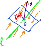
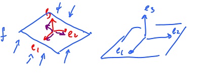
The projection of the plane onto line $l$ is illustrated below left. Then, of course, the image is $l$:

$${\rm Im}(f) = l.$$

But another interesting subset is the kernel of $f$:

$${\rm ker}(f) = \{x \colon f(x) = 0 \}.$$

In other words this is the preimage of $0$. It is illustrated center and right.

Definition.

The kernel of $f$ is $\{x: f(x) = 0 \}$.
The nullity of $f$ is the dimension of the kernel of $f$.

Theorem. The kernel of $f$ is a linear subspace.

Proof. Suppose

$$x_1, x_2 \in ker(f).$$

Consider

$$f(x_1 + x_2) = f(s_1) + f(x_2) = 0 + 0 = 0, {\rm \hspace{3pt} so}$$

$$x_1 + x_2 \in ker(f). {\rm \hspace{3pt} QED}$$

Exercise. What about scalar multiplication?

Keep in mind the main difference between these two linear spaces. If

$f \colon {\bf R}^n \rightarrow {\bf R}^m$ is a linear function,

the kernel is in the domain while the image is in the target:

$${\rm ker}(f) \subset {\bf R}^n,$$

$${\rm Im}(f) \subset {\bf R}^m.$$

Example. Consider the projection of ${\bf R}^3$ onto a plane $P$. The kernel is the line through $0$, perpendicular to $P$. Then

$${\rm Im}(f) = P, {\rm dim \hspace{3pt}} P = 2;$$

$${\rm ker}(f) = l, {\rm dim \hspace{3pt}} l = 1.$$

Observe that

$2 + 1 = 3 =$ dimension ${\bf R}^3$.

More generally, for

$$f \colon {\bf R}^n \rightarrow {\bf R}^n,$$

Definition.

• The dimension of the kernel $f$ is called the nullity of $f$, $N(f)$;
• The dimension of the image $f$ is called the rank of $f$, ${\rm rank}(f)$.

Theorem.

$$N(f) + {\rm rank}(f) = n.$$

Then the possible images/kernels are arranged according to this split of $n$. For example for $$f: {\bf R}^2 \rightarrow {\bf R}^2$$

we have

$${\rm Im}(f) = 0, {\rm ker}(f) = {\bf R}^2;$$

${\rm Im}(f) =$ line, ${\rm ker}(f) =$ line;

$${\rm Im}(f) = {\bf R}^2, {\rm ker}(f) = 0.$$

Theorem. If $x_1, \ldots, x_s$ span $A$, then $f(x_1), \ldots, f(x_s)$ span $f(A)$.

Observe that even if $x_1, \ldots, x_s$ is a basis, $f(x_1), \ldots, f(x_s)$ does not have to be. Linear independence may be lost under $f$.

Example.

• $f(e_1) = e_1$;
• $f(e_2) = e_2$;
• $f(e_3) = 0$;
• $\{e_1, e_2, 0 \}$ is linear dependent.

Q: Suppose $x_1, \ldots, x_s$ is a basis of $A$, when is $f(x_1), \ldots, f(x_s)$ a basis of $f(A)$?

A: ${\rm ker}(f) = 0$. Because in this case ${\rm rank}(f) = s$.

If ${\rm ker}(f) \neq 0$, then ${\rm Im}(f) \neq {\bf R}^s$.

Recall the graph of a function

$$y = f(x), f \colon {\bf R} \rightarrow {\bf R} $$

is defined as

$${\rm Gr}(f) = \{(x,f(x)) \colon x\in{\bf R} \}.$$

For $f \colon {\bf R}^n \rightarrow {\bf R}^m$, the definition is the same:

$${\rm Gr}(f) = \{(x,f(x)) \colon x\in{\bf R}^n \}.$$

Since

$$x \in {\bf R}^n, f(x) \in {\bf R}^m,$$

we have

$${\rm Gr}(f) \subset {\bf R}^{n+m}.$$

Example. Consider

$$f(x,y,z)=(x+y,x-z), u=(x,y,z).$$

Then

$$(u,f(u)) = (x, y, z, x + y, x - z) \in {\bf R}^5.$$

Theorem. The graph of a linear function $f, {\rm Gr}(f)$, is a linear subspace.

Proof. Exercise.

Solution sets of linear equations

The simplest linear equation:

$f(x) = b$, find $x$.

What is the solution set? It is not a linear subspace.

Dimension $1$.

$f(x)=3x$ in ${\bf R}^3$.

Solve $3x=5$.

Answer: a (no-zero) point, $x = 5/3$.

Dimension 2. $f(x,y) = x + y$ for $f \colon {\bf R}^2 \rightarrow {\bf R}$.

Solve $f(x,y) = 5$.

Answer: $x + y = 5$, a line (not through $0$).

Theorem.

1. The solution set $A$ of a linear equation $f(x) = b$ is an affine subspace.
2. The solution set of a homogeneous linear equation $f(x) = 0$ is the kernel of $f$, hence a linear subspace.

• $f(x) = 0$ is a homogeneous equation;
• $f(x) = b$ is non-homogeneous equation.

Special case.

$$f \colon {\bf R}^n \rightarrow {\bf R} (m=1)$$

called linear functionals.

$$f(x) = y, x \in {\bf R}^n, y \in {\bf R};$$

$$f(x) = a_1x_1 + a_2x_2 + ... + a_nx_n = <a,x>, $$

where $a = (a_1, a_2, ..., a_n)$.

Theorem. Every linear functional $f$ corresponds to a vector $a$ such that

$$f_a(x) = <a,x>,$$

and vice versa.

The algebra of linear maps

Linear functions form a linear subspace.

First, the set of all (not necessarily linear) functions $$f: {\bf R}^n \rightarrow {\bf R}^n$$ form a linear space. Consider $f(x,y)$ or $g(x,y)$.

These are the operations:

• $f + g: {\bf R}^2 \rightarrow {\bf R}^2$ the sum;
• ${\alpha}f: {\bf R}^2 \rightarrow {\bf R}^2$ the scalar product.

Consider now the set of all linear functions $f: {\bf R}^n \rightarrow {\bf R}^m, n$ and $m$ are fixed, denoted as $L(n,m)$.

Vector operations.

What is the sum? $$f,g \in L(n,m), f + g = ?$$ Define it as: $$(f + g)(x) = f(x) + g(x).$$

What is the scale product? $$f \in L(n,m), {\alpha} \in {\bf R}, {\alpha}f = ?$$ Define it as: $$({\alpha}f)(x) = {\alpha} \cdot f(x).$$

What is the $0$ element in $L(n,m)$? Define it as: $$0: {\bf R}^n \rightarrow {\bf R}^m: $$ $$0(x) = 0 {\rm \hspace{3pt} for \hspace{3pt} all \hspace{3pt}} x.$$

Exercise. Verify the properties.

Theorem. $${\rm dim \hspace{3pt}}L(n,m) = n \cdot m.$$ (Like ${\bf R}^{nm}$.)

Proof. Matrices... $\blacksquare$

Example.

$n = 1, m = 1$, thus $n \cdot m = 1$;

Indeed, all linear functions are simply $$f(x) = mx,$$ so that $$f \longleftrightarrow m \in {\bf R}.$$

Special case $n = m$. In this case, for all functions $$f,g: {\bf R}^n \rightarrow {\bf R}^n$$ we can also form compositions: $$f,g \in L(n,n) \rightarrow fg \in L(n,n).$$

Addition and scalar multiplication, then $L(n,n)$ is a linear space. Addition, scalar multiplication, and composition, then $L(n,n)$ is an "algebra":

• ${\alpha}(fg) = f({\alpha}g)$, as $f, g$ are linear;
• $f(g + h) = fg + fh$, as $f,g$ and $h$ are linear.

(Notation: $f \circ g$ instead of $fg$.)

Compositions of linear functions are realized via matrix multiplication.

Definition. Suppose $f: {\bf R}^n \rightarrow {\bf R}^m$, $g: {\bf R}^m \rightarrow {\bf R}^k$ are linear. Then the composition is $$gf: {\bf R}^n \rightarrow {\bf R}^k$$ defined by $$(gf)(x) = g(f(x)).$$

$$ \newcommand{\ra}[1]{\!\!\!\!\!\!\!\xrightarrow{\quad#1\quad}\!\!\!\!\!} \newcommand{\da}[1]{\left\downarrow{\scriptstyle#1}\vphantom{\displaystyle\int_0^1}\right.} % \begin{array}{cccccc} {\bf R}^n & \ra{f} & {\bf R}^m & \ra{g} & {\bf R}^k \\ x & \longmapsto & y=f(x) & \longmapsto & z=g(y) \\ \end{array} $$

You can see what happens in this diagram:

Properties.

Linearity = additivity + homogeneity.

The commutative diagram below shows how compositions respect scalar products:

$$ \newcommand{\ra}[1]{\!\!\!\!\!\!\!\xrightarrow{\quad#1\quad}\!\!\!\!\!} \newcommand{\da}[1]{\left\downarrow{\scriptstyle#1}\vphantom{\displaystyle\int_0^1}\right.} % \begin{array}{cccccc} {\bf R}^n & \ra{\alpha f} & {\bf R}^m & \ra{g} & {\bf R}^k \\ & \searrow ^f & & \nearrow ^ {\alpha g}\\ & &{\bf R}^m & \end{array} $$

• Homogeneity: $g({\alpha}f) = ({\alpha}g)f$;
• Additivity: $(g + h)f = gf + hf$;
• Distributivity, left: $g(f+l) = gf + gl$;
• Distributivity, right: $(f+l)g = fg + lg$.

In general, $fg \neq gf$, no commutativity.

Indeed, on one hand $$\left| \begin{array}{} 1 & 2 \\ 3 & 4 \end{array} \right| \left| \begin{array}{} 2 & 1 \\ 3 & 4 \end{array} \right| = \left| \begin{array}{} 8 & * \\ * & * \\ \end{array} \right|$$ On the other hand $$\left| \begin{array}{} 2 & 1 \\ 3 & 4 \end{array} \right| \left| \begin{array}{} 1 & 2 \\ 3 & 4 \end{array} \right| = \left| \begin{array}{} 5 & x \\ * & * \\ \end{array} \right|$$

Not equal!

Identity element. There are left and right identity $I\in L(m,m)$ and $J\in L(n,n)$ ,so that for all $f$:

• $If = f$:

$$ \newcommand{\ra}[1]{\!\!\!\!\!\!\!\xrightarrow{\quad#1\quad}\!\!\!\!\!} \newcommand{\da}[1]{\left\downarrow{\scriptstyle#1}\vphantom{\displaystyle\int_0^1}\right.} % \begin{array}{llllllllllll} & {\bf R}^n & \ra{f} & {\bf R}^m \\ & \da{J} & \nearrow _f & \\ & {\bf R}^n & & \end{array} $$

• $fJ = f:$

$$ \newcommand{\ra}[1]{\!\!\!\!\!\!\!\xrightarrow{\quad#1\quad}\!\!\!\!\!} \newcommand{\da}[1]{\left\downarrow{\scriptstyle#1}\vphantom{\displaystyle\int_0^1}\right.} % \begin{array}{llllllllllll} & {\bf R}^n & \ra{f} & {\bf R}^m \\ & & \searrow ^{f} & \da{I} \\ & & & {\bf R}^m \end{array} $$

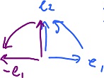
Exercise. Consider a linear function with $$A(e_1) = e_2;$$

$$A(e_2) = -e_1.$$

Then $$\begin{array}{} A({\alpha}e_1 + {\alpha}_2e_2) &= {\alpha}_1A(e_1) + {\alpha}_2A(e_2) &= {\alpha}_1e_2 - {\alpha}_2e_1 &= -{\alpha}_2e_1 + {\alpha}_1e_2. \end{array}$$

This is a rotation! (What is its matrix?)

Observe:

Rotation $\cdot$ flip $\neq$ flip $\cdot$ rotation.

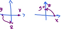
In the image, the rotation is $90$ degrees and the flip is about the $y$-axis.

In the next example, we consider the composition of the same rotation with the reflection about the origin. Then

Rotation $\cdot$ reflection $=$ reflection $\cdot$ rotation.

Indeed, let $R_x$ denote the rotation through $x$ degrees, then $$R_{90}R_{180} = R_{270} = R_{180}R_{90}.$$ No commutativity in this case.

Observe that $$R_{90} + R_{180}$$ is not a rotation!

Exercise. Is $L(2,2)$ a linear space with respect to composition (instead of addition)?

More on matrices

Review exercise. Let $$f(x_1, x_2) = (x_1 - x_2, x_1 + 2x_2)$$ It is represented by the matrix $$A = \left| \begin{array}{} \ldots & \ldots \\ \ldots & \ldots \end{array} \right|$$

What is it?

$$AX = A = \left| \begin{array}{} \ldots & \ldots \\ \ldots & \ldots \end{array} \right| \left| \begin{array}{} x_1 \\ x_2 \end{array} \right| = (x_1 - x_2, x_1 + 2x_2)$$

We just fill the blanks in the matrix by examining what we need to have in the right hand side vis matrix multiplication:

$$\left| \begin{array}{r} 1 & -1 \\ 1 & 2 \end{array} \right| \left| \begin{array}{} x_1 \\ x_2 \end{array} \right| = (x_1 - x_2, x_1 + 2x_2)$$

More generally, $$A = \left| \begin{array}{} a_{11} & a_{12} \\ a_{21} & a_{22} \end{array} \right|$$ where $$a_{11}=1; a_{12}=-1; a_{21}=1; a_{22}=2.$$

Suppose $A: {\bf R}^n \rightarrow {\bf R}^m$ is a linear function. Then it is represented by a $m \times n$ matrix.

For example, let $g(y_1, y_2) = (y_1, y_1 + Y_2); g: {\bf R}^2 \rightarrow {\bf R}^2.$

Then its matrix is $$\left| \begin{array}{} 1 & 0 \\ 1 & 1 \end{array} \right|$$

Next $gf: {\bf R}^2 \rightarrow {\bf R}^2;$ $$\begin{array}{} gf(x_1, x_2) &= g(x_1 - x_2, x_1 + 2x_2) \\ &= (x_1 - x_2, (x_1 - x_2) + (x_1 + 2x_2)) \\ &= (1(x_1 - x_2) + 0(x_1 - {\alpha}x_2), 1(x_1 - x_2) + 1(x_1 + 2x_2). \end{array}$$

This explains why matrices are multiplied the way they are: $$A = \left| \begin{array}{r} 1 & -1 \\ 1 & 2 \end{array} \right|$$

$$\left| \begin{array}{} 1 & 0 \\ 1 & 1 \end{array} \right|$$

Notice the difference in the dimensions of the matrices involved:

• Addition: $A_{n \times m} + B_{n \times m} = C_{n \times m}$;
• Multiplication: $A_{n \times m} \cdot B_{m \times k} = C_{n \times k}$

$f(x) = mx$ - linear function;
$g(x) = mx + b$ – affine function.

More generally,

Definition. A function $g: {\bf R}^n \rightarrow {\bf R}^m$ is called affine if there are a linear function $f \colon {\bf R}^n \rightarrow {\bf R}^m$ and a constant vector $b \in {\bf R}^m$ such that

$$g(x) = f(x) + b.$$

Properties. Linear:

1. Image of f is a linear subspace;
2. Kernel of f is a linear subspace;
3. Graph of f is a linear subspace.

Affine:

1. Image of g is an affine subspace;
2. Kernel of g is an affine subspace;
3. Graph of g is an affine subspace.