Derivative reflects behavior of the function

We consider some theory about how one can find out about the behavior of the function from its derivative.

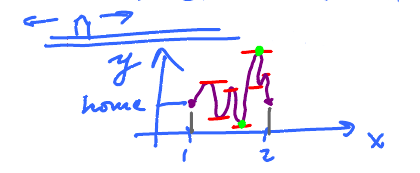
Imagine that you:

• left home at 1pm,
• did some driving,
• came home at 2 pm.

Question: What can you say about your speed during this time?

For simplicity we assume that you drove on a straight road...

You may have driven slower and faster but this is the main thing: you came back home.

And to come back you had to turn around. To turn around you had to stop.

So, speed = 0 at least once!

Let's make this observation more mathematical and turn it into a theorem.

Let $x$ be time, limited to interval $[a,b]$, and $y=f(x)$ be your location at time $x$. Then speed/velocity corresponds to the derivative $f'$ of the function.

Theorem.

1. $f$ is given, defined on $[a,b]$,
2. $f$ is continuous on $[a,b ]$,
3. $f$ is differentiable on $(a,b)$,
4. $f(a) = f(b)$.

Then $f^{\prime}(c) = 0$ for some $c$ in $[a,b]$.

This is called Rolle's Theorem.

In the theorem, #2 means that you don't leap, #3 means that the velocity makes sense, #4 "I came back".

How do we prove it? What is this special point in time?

Consider the moment when you were farthest away from home (in either direction). That's the idea: you weren't moving then.

Proof.

Suppose $f$ has

• a global max at $x = c$ and
• a global min at $x = d$.

These assumptions are justified by the Extreme Value Theorem. ($\Rightarrow$ need continuity).

Recall Fermat's theorem:

• if $c$ is a local max them $f^{\prime}(c) = 0$.
• If $d$ is a local max then $f^{\prime}(c) = 0$.

We use the fact that every global max/min is a local max/min unless it's an end point.

Case 1. Neither $c$ nor $d$ is an end point, $a$ or $b$.

Then $f^{\prime}(c) = 0$ or $f^{\prime}(d) = 0$, done. (here $c$ or $d$ is in $(a,b)$).

Case 2. Both $c$ and $d$ are the end points, $a$ or $b$.

Then $$\left.\begin{aligned} f(c) & = f(a) \qquad \text{ or } \qquad f(c) = f(b) \\ f(d) & = f(a) \qquad \text{ or } \qquad f(d) = f(b) \end{aligned} \right\} \qquad \text{But these are equal!} $$ So, $$f(c) = f(d).$$ But this means that max=min!

Therefore $f$ is constant, so $f^{\prime}(x) = 0$ for all $x$. $\blacksquare$

This is important result but, generally, we don't expect to have $f(a) = f(b)$ (coming home). Let's generalize this result.

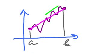
If we rotate the picture above, the result might look like this:

The picture suggests what happens to the entities we considered in Rolle's theorem:

• The tangents of those special points used to be horizontal and now they have become inclined.
• The line that connects the end points used to be horizontal and now is has become inclined.

But these lines are still parallel!

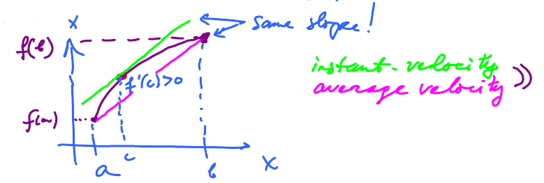
So, we need to find a connection between

• $f^{\prime}$ on $(a,b)$ (that's the velocity) and
• the slope of the line between $(a,f(a))$ and $(b,f(b))$ (that's the average velocity on $[a,b]$).

In terms of motion, this is what we see:

$\underbrace{f^{\prime} > 0}_{\text{Direction of motion is to the right.}}$ on $[a,b]$, so $\underbrace{f(b) > f(a)}_{\text{I moved to the right.}}$.

Graphically 

To illustrate, let's revisit the radar gun issue.

Radar gun catches the instantaneous velocity of the car. By law it shouldn't be above 70 m/h. When the radar gun shows anything above, you're caught.

Now, suppose there is no radar gun. Imagine instead a cop observed you in Huntington and then, after 30 minutes, in Charleston, 50 miles away.

Then the average speed of yours was 100 m/h. Bad, but did you violate the law?

The analysis we pursue here allows one to infer that yes, your instantaneous velocity was 100 m/h at some point. So, you were speeding!

Mean Value Theorem. Suppose

• $f$ is given on $[a,b]$,
• $f$ is continuous on $[a,b]$,
• $f$ is differentiable on $[a,b]$.

Then $$\underbrace{\frac{f(b) – f(a)}{b-a}}_{\text{The slope of the secant line, }g(x)} = f^{\prime}(c)$$ for some $c$ in $[a,b].$

In the equation:

• LHS = average velocity and
• RHS = instantaneous velocity over $[a,b]$ which is

$$ \frac{\text{displacement}}{\text{time}} $$

What happens if in MVT, $f(a) = f(b)$?

Then LHS = 0, then $0 = f^{\prime}( c)$. We have the conclusion of Rolle's Theorem. So, MVT is more general than RT. In other words, the latter is an instance, a narrow case of MVT.

How do we prove it?

Let's compare MVT and RT.

We rename $f$ as $h$ to use it later. Then the conditions of Rolle's Theorem look like this:

• $h$ is given, defined on $[a,b]$.
• $h$ is continuous on $[a,b]$.
• $h$ is differentiable on $[a,b]$.
• $ h(a) = h(b) $.

Let' also look at the graphs:

Note 1 

In either case we are after $c$ with $f^{\prime}(c)$ equal the slope of the secant line.

Note 2 

Graphs are similar.

Define $g(x)$ as the function represented by the secant line. We can only apply RT, to $h$ with $$ h(a) = h(b). $$ Unfortunately, $f$ is not like that.

Smart idea: let's try this. $$ h(x) = f(x) – g(x).$$ Since $$\begin{aligned} f(a) &= g(a) \\ f(b) &= g(b), \end{aligned}$$ it follows $$\begin{aligned} h(a) &= 0, \\ h(b) &= 0, \\ \Rightarrow h(a) &= h(b) \end{aligned}$$ This fits RT!

Next, $h$ is continuous on $[a,b]$ as the difference of the two continuous functions.

Also, $h$ is differentiable on $(a,b)$ as the difference of the two differentiable functions.

Thus $h$ satisfies the conditions of RT. Therefore the conclusion is satisfied too: $$\underbrace{h^{\prime}(c) = 0}_{\text{substitute } f,g \text{ to get MVT.}}$$ for some $c$ in $(a,b)$

We need a formula for $g$ now.

It's a straight line and its slope is $$ m = \frac{f(b) – f(a)}{b-a}, \qquad g \text{ is linear}.$$ Use the point-slope formula $$\begin{aligned} y – y_{0} &= m(x - x_{0}), \quad \text{or}\\ g(x) &= y_{0} + m(x – x_{0}) \end{aligned}$$ then $$g(x) = f(a) + m(x – a).$$ Then $$\begin{aligned} h(x) &= f(x) – g(x) \\ &= f(x) – f(a) - m(x – a). \end{aligned}$$ So $$\begin{aligned} h^{\prime}(x) & = f^{\prime}(x) - 0 - m, \quad \text{or} \\ h^{\prime}(x) &= f^{\prime}(x) - m \end{aligned}$$ By RT, $$ h^{\prime}(c) = 0 $$ for some $c$, so $$\begin{aligned} f^{\prime}(c) – m &= 0 \quad \text{or} \\ f^{\prime}(c) &= m. \end{aligned}$$ That's the LHS of MVT. $\blacksquare$

Meaning of the theorem

$$\text{Derivative at } c = \text{Slope of the secant line}$$

$$\text{instantenous veliocity at some point in time} = \text{Average Velocity}$$

Example: If 100 miles covered in 1 hour, then was speeding at some point.

Consider this simple statement about motion:

"if my velocity is zero, I am standing still". 

Suppose $f$ is the position, restate this mathematically.

Corollary. If $$f^{\prime}(x) = 0 \, \forall x$$ on an interval $(A,B)$, then $f$ is constant on $(A,B)$.

Proof. To prove that $f$ is constant, it suffices to show that $$f(a) = f(b)$$ for all $a,b$ in $(A,B)$.

Assume $a < b$ and use MVT ($(a,b) \subset (A,B)$): $$\frac{f(b) – f(a)}{b-a} =\begin{cases} f^{\prime}(c) & \text{for some } c \text{ in } (a,b) \\ =0 & \text{ny assumption, for all } c \text{ in } (a,b) \subset (A,B) \end{cases}$$ So $$\frac{f(b) - f(a)}{b-a} = 0$$ always. (Observe $(b-a) \neq 0$ as $b > a$.)

Hence $$f(b) – f(a) = 0$$ or $$f(a) = f(b).$$ $\blacksquare$

Let's take the opposite route this time. We state a theorem and then interpret it in terms of motion.

Corollary. If $$f^{\prime}(x) = g^{\prime}(x)$$ $\forall x$ in $(A,B)$, then $$f(x) – g(x)$$ is constant.

Geometrically, this means that the graphs are shifted vertically.

Restated for motion:

"If two runners run with the same speed, the distance between them isn't changing". 

It's as if they are tied by a rope that will never break or hang.

Proof. Idea, define $$h(x) = f(x) – g(x).$$ Then $$\begin{aligned} h^{\prime}(x) &= (f(x) –g(x))^{\prime} \\ =f^{\prime}(x) –g^{\prime}(x) \\ =0, \forall x. \end{aligned}$$ Then $h$ is constant, by the previous corollary. $\blacksquare$

See Using derivative to study monotonicity.