This site is being phased out.
Vector functions
Contents
- 1 Introduction
- 2 Plotting the function as a transformation of the grid
- 3 Plotting the function as a vector field
- 4 Plotting the image of the function
- 5 Tangent plane and the total derivative
- 6 Differentiation
- 7 The Mean Value Theorem
- 8 Proof of the Chain Rule
- 9 Parametrized hypersurfaces
- 10 Level sets
Introduction
We have considered two types of "vector functions":
- parametric curves as functions $f: {\bf R} {\rightarrow} {\bf R}^m$ and
- functions of several variables as functions $f: {\bf R}^n {\rightarrow} {\bf R}$.
These are very different objects with very different issues to consider.
Now it's time too consider the general vector functions, i.e., both input and output are vector:
$$f: {\bf R}^n {\rightarrow} {\bf R}^m,$$
A simple example is that of a linear operator which graph is hyperplane in ${\bf R}^{n+m}$.
Suppose $f: {\bf R}^n {\rightarrow} {\bf R}^m$ is a continuous function at a fixed $x = a$. In the $1$-dimensional case this means that for any $\epsilon > 0$ there is a $\delta > 0$ such that for
$$| x - a | < \delta$$
follows
$$| f(x) - f(a) | < \epsilon.$$
If $n, m > 1$, simply replace $| \cdot |$ with $|| \cdot ||$.
In the $1$ dim case there are $4$ algebraic operations that preserve continuity. Some of them don't apply to the $n$ dim case:
- no division $\frac{f(x)}{g(x)}, f, g: {\bf R}^n {\rightarrow} {\bf R}^m$,
- no multiplication $f(x) \cdot g(x), f, g: {\bf R}^n {\rightarrow} {\bf R}^m$, unless these are scalar functions $f(x) \cdot g(x), f: {\bf R}^n {\rightarrow} {\bf R}, g: {\bf R}^n {\rightarrow} {\bf R}^m$, or it's
the dot product $< f(x), g(x) > = f(x) \cdot g(x): {\bf R}^n {\rightarrow} {\bf R}$,
- etc.
Plotting the function as a transformation of the grid
As we have to limit ourselves to ${\bf R}^3$, only the image of a function from ${\bf R} {\rightarrow} {\bf R}^m$ for any $m \leq 3$ can be visualized and the graph of a function from ${\bf R}^n {\rightarrow} {\bf R}$ can be visualized only for $n \leq 2$.
Indeed, consider a function $f: {\bf R}^n {\rightarrow} {\bf R}^m$. Since the graph lies in ${\bf R}^{n+m}$, we have to have
$$( n + m ) \leq 3, {\rm \hspace{3pt} i.e. \hspace{3pt}} ( n , m ) = ( 1, 2 ) {\rm \hspace{3pt} or \hspace{3pt}} ( 2, 1 ).$$
What about $n = m = 2$? This kind of function can be interpreted as a transformation of the plane:
$$f: {\bf R}^n {\rightarrow} {\bf R}^m$$
$$(y_1, y_2) = f(x_1, x_2). $$
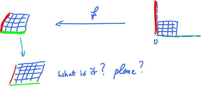
One way to visualize what the function does is to
- Plot a square $s$ in the $x_1,x_2$-plane and then
- plot the image of $s$ in the $y_1,y_2$-plane.
For a more complete picture, consider the image of a rectangular grid:
Example. Let $f( x_1, x_2 ) = ( 1 - x_1 + 2x_2, 3 - 2x_1 + x_2 )$. Then
$$f( 0, 0 ) = ( 3, 1), f( 1, 1 ) = ( 2, 2).$$
Where do the horizontal lines go? Plug in $y_2 = b$ into $f$ (with $t {\in} {\bf R}, b$ fixed):
$$\begin{array}{} f( t, b ) &= ( 1 - t + 2b, 3 - 2t + b ), {\rm \hspace{3pt} (point \hspace{3pt} on \hspace{3pt} the \hspace{3pt}} y_1y_2{\rm-plane}) \\ &= ( 1 + 2b, 3 + b ) + t ( -1, -2 ) {\rm \hspace{3pt} (straight \hspace{3pt} line).} \end{array}$$
For $b = 0$, this yields
$$f( t, 0 ) = ( 1, 3 ) + t ( -1, -2 ).$$
For $b = 1$, this yields
$$f( t, 1 ) = ( 3, 4 ) + t ( -1, -2 ).$$
Where do the vertical lines go? Plug in $x_1 = a$ into $f$:
$$\begin{array}{} f( a, s ) &= ( 1 - a + 2s, 3 - 2a + s) &= ( 1 - a, 3 - 2a ) + s ( 2, 1 ). \end{array}$$
For $a = 0$, this yields
$$f( 0, s ) = ( 1, 3 ) + s ( 2, 1 ).$$
This is the end result:
Since $f$ is an affine function, the straight lines remain straight lines.
Plotting the function as a vector field
Another way to visualize such a function is to treat it as a the vector field.
Even though the input and the output of $f: {\bf R}^2 {\rightarrow} {\bf R}^2$ are of the same nature, a pair of numbers, they can be differently interpreted. A pair of numbers can be a point on the plane (input) or it can be a vector on the plane (output). So, the function assigned a vector to every point:
Then, we attach $f(x)$ to $x$.
The result is a "field" of vectors.
The easiest way to think about this construction is as if $x$ is a particle and it moves to $x + f(x)$.
Example. Consider the same function:
$$f( x_1, x_2 ) = ( 1 - x_1 + x_2, 3 - 2x_1 + x_2 ),$$
where
$x = ( x_1, x_2 )$ a point.
To plot $f$, we list the input first - in the first two columns, then the corresponding output in the last two columns. Then we plot the output vector starting at the input point.
For more see Vector fields.
Plotting the image of the function
Plotting just the image of the function $f: {\bf R}^n {\rightarrow} {\bf R}^m$, may be the only option for $m>2$.
Under certain circumstances and if $n < m$, the image ${\rm im}(f)$ is a $n$-dimensional manifold in ${\bf R}^m$.
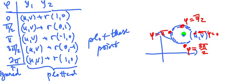
Example. Define $f: {\bf R} {\rightarrow} {\bf R}^2$ by
$$\begin{array}{} f( {\varphi} ) &= ( u + r {\rm cos \hspace{3pt}} {\varphi}, v + r {\rm sin \hspace{3pt}} {\varphi} ) \\ &= ( u, v ) + r ( {\rm cos \hspace{3pt}} {\varphi}, {\rm sin \hspace{3pt}} {\varphi} ), {\varphi} {\in} [ 0, 2 \pi ]. \end{array}$$
This is a parametric curve the image of which is a circle with center $( u, v )$, radius $r$, while $( {\rm cos \hspace{3pt}} {\varphi}, {\rm sin \hspace{3pt}} {\varphi} )$ is the angle. Plot the image of $f$:
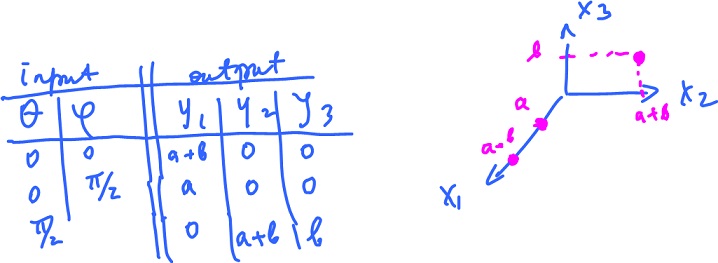
Example. Surface in space. Define $f: {\bf R}^2 {\rightarrow} {\bf R}^3$ by
$$f( {\theta}, {\varphi} ) = ( ( a + b {\rm cos \hspace{3pt}} {\varphi} ) {\rm cos \hspace{3pt}} {\theta}, ( a + b {\rm cos \hspace{3pt}} {\varphi} ) {\rm sin \hspace{3pt}} {\theta}, b {\rm sin \hspace{3pt}} {\varphi} ).$$
Domain: ${\theta} {\in} [ 0, 2 {\pi} ), {\varphi} {\in} [ 0, 2 {\pi} ]$. Plot point by point:
Too few point to understand what this is. But it is, in fact, a torus. Then we can think of it and plot as a "parametric surface". Indeed we rotate a circle (off center) in the $yz$-plane around the $z$-axis:
Let's explain where this construction comes from. Consider the formula again:
$$f( {\theta}, {\varphi} ) = ( ( a + b {\rm cos \hspace{3pt}} {\varphi} ) {\rm cos \hspace{3pt}} {\theta}, ( a + b {\rm cos \hspace{3pt}} {\varphi} ) {\rm sin \hspace{3pt}} {\theta}, b {\rm sin \hspace{3pt}} {\varphi} ).$$
1. Fix ${\theta} = 0$, find the image with one parameter (parametric curve).
$$\begin{array}{} f( 0, {\varphi} ) &= ( ( a + b {\rm cos \hspace{3pt}} {\varphi} ) {\rm cos \hspace{3pt}} 0, ( a + b {\rm cos \hspace{3pt}} {\varphi} ) {\rm sin \hspace{3pt}} 0, b {\rm sin \hspace{3pt}} {\varphi} ) \\ &= ( a + b {\rm cos \hspace{3pt}} {\varphi}, 0, b {\rm sin \hspace{3pt}} {\varphi} ) &= ( a, 0, 0 ) + b ( {\rm cos \hspace{3pt}} {\varphi}, 0 {\rm sin \hspace{3pt}} {\varphi} ). \end{array}$$
What is it? A circle in the $y_1y_3$-plane with center $( a, 0, 0 )$ and radius $b$. Fix ${\theta} = 2{\pi}$, find the image.
$$\begin{array}{} f( 0, {\varphi} ) &= ( ( a + b {\rm cos \hspace{3pt}} {\varphi} ) {\rm cos \hspace{3pt}} 2{\pi}, ( a + b {\rm cos \hspace{3pt}} {\varphi} ) {\rm sin \hspace{3pt}} 2{\pi}, b {\rm sin \hspace{3pt}} {\varphi} ) \\ &= ( a + b {\rm cos \hspace{3pt}} {\varphi}, 0, b {\rm sin \hspace{3pt}} {\varphi} ), \end{array}$$
no change to previous calculation as $2{\pi}$ is the period of the ${\rm sin \hspace{3pt}}$ and the ${\rm cos \hspace{3pt}}$.
2. Fix ${\varphi} = 0$, find the image with one parameter.
$$\begin{array}{} f( {\theta}, 0 ) &= ( ( a + b {\rm cos \hspace{3pt}} 0 ) {\rm cos \hspace{3pt}} {\theta}, ( a + b {\rm cos \hspace{3pt}} 0 ) {\rm sin \hspace{3pt}} {\theta}, b {\rm sin \hspace{3pt}} 0 ) \\ &= ( ( a + b ) {\rm cos \hspace{3pt}} {\theta}, ( a + b ) {\rm sin \hspace{3pt}} {\theta}, 0 ). \end{array}$$
What is it? A circle in the $y_1y_2$-plane with center $( 0, 0, 0 )$ and radius $( a + b )$.
For more see Torus.
Tangent plane and the total derivative
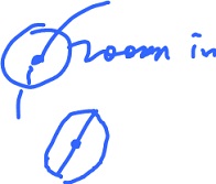
We are now interested in the "local" behavior of these functions. What does the graph look like if we zoom in on a particular point?
In Calc 1, the answer is "tangent line'" for functions of one variable. Same for parametric curves. For functions of several variables, it is "hyperplane".
In the last case the answer is this simple because, typically, the graph of a function $f: {\bf R}^n {\rightarrow} {\bf R}$ is an $n$-dimensional manifold in ${\bf R}^{n+1}$. It is slightly trickier in the case of vector functions since the graph of $f: {\bf R}^n {\rightarrow} {\bf R}^m$ is an $n$-dimensional manifold in ${\bf R}^{n+m}$.
Let's try to visualize the local behavior of such a function. Since the function is a transformation of the plane, we'll zoom in on its image. The image is a surface but what happens as we zoom in?
What is is? It is the tangent plane, i.e. the image of the best affine approximation. It is found by means the Jacobian of $f$.
Example. Let's consider the torus again. It is represented by
$$f: {\bf R}^2 {\rightarrow} {\bf R}^3$$
The function has $6$ partial derivatives, as $6 = 3 {\times} 2$.
$$f( {\theta}, {\varphi} ) = ( ( a + b {\rm cos \hspace{3pt}} {\varphi} ) {\rm cos \hspace{3pt}} {\theta}, ( a + b {\rm cos \hspace{3pt}} {\varphi} ) sin {\theta}, b {\rm sin \hspace{3pt}} {\varphi} ),$$
decompose:
$$f_1( {\theta}, {\varphi} ) = ( a + b {\rm cos \hspace{3pt}} {\varphi} ) {\rm cos \hspace{3pt}} {\theta},$$
$$f_2( {\theta}, {\varphi} ) = ( a + b {\rm cos \hspace{3pt}} {\varphi} ) {\rm sin \hspace{3pt}} {\theta},$$
$$f_3( {\theta}, {\varphi} ) = b {\rm sin \hspace{3pt}} {\varphi}.$$
These are the partial derivatives:
$$f'_1: \frac{\partial f_1}{\partial {\theta}} = -( a + b {\rm cos \hspace{3pt}} {\varphi} ) {\rm sin \hspace{3pt}} {\theta}, \frac{\partial f_1}{\partial {\varphi}} = -b {\rm sin \hspace{3pt}} {\varphi} {\rm cos \hspace{3pt}} {\theta} ( \leftarrow {\nabla} f_1 )$$
$$f'_2: \frac{\partial f_2}{\partial \theta} = ( a + b {\rm cos \hspace{3pt}} {\varphi} ) {\rm cos \hspace{3pt}} {\theta}, \frac{\partial f_2}{\partial {\varphi}} = -b {\rm sin \hspace{3pt}} {\varphi} {\rm sin \hspace{3pt}} {\theta} ( \leftarrow {\nabla} f_2 )$$
$$f'_3: \frac{\partial f_3}{\partial \theta} = 0, \frac{\partial f_3}{d{\varphi}} = b {\rm cos \hspace{3pt}} {\varphi} ( \leftarrow {\nabla} f_3 )$$
Hence the total derivative can be written as a matrix called the Jacobian:
$$f'( {\theta}, {\varphi} ) = \left| \begin{array}{} -( a + b {\rm cos \hspace{3pt}} {\varphi} ) {\rm sin \hspace{3pt}} {\theta} & -b {\rm sin \hspace{3pt}} {\varphi} {\rm cos \hspace{3pt}} {\theta} \\ ( a + b {\rm cos \hspace{3pt}} {\varphi} ) {\rm cos \hspace{3pt}} {\theta} & -b {\rm sin \hspace{3pt}} {\varphi} {\rm sin \hspace{3pt}} {\theta} \\ 0 & b {\rm cos \hspace{3pt}} {\varphi} \end{array} \right|$$
The best affine approximation of $f(x)$ at $x = a$ is
$$T(x) = f(a) + f'(a) ( x - a ),$$
where
$$x {\in} {\bf R}^2, T(x) {\in} {\bf R}^3,$$
$$a {\in} {\bf R}^2, f(a) {\in} {\bf R}^3,$$
$f'(a)$ is a matrix of dimension $3 {\times} 2$,
$$( x - a ) {\in} {\bf R}^2.$$
Let's find the best approximation for our torus at $a = ( 0, 0, 0 )$.
$$f(a) = f( 0, 0 ) = ( a + b, 0, 0 ).$$
Here
$$f'(a) = \left| \begin{array}{} 0 & 0 \\ a + b & 0 \\ 0 & b \end{array} \right|$$
Define $T: {\bf R}^2 {\rightarrow} {\bf R}^2$ as
$$\begin{array}{} T( {\theta}, {\varphi} ) &= ( a + b, 0, 0 )^T + \left| \begin{array}{} 0 & 0 \\ a+b & 0 \\ 0 & b \end{array} \right| \cdot ( [ {\theta}, {\varphi} ]^T - [ 0, 0 ]^T ) \\ &= ( a + b, 0, 0 )^T + ( 0, ( a + b ) {\theta}, b{\varphi} )^T \\ &= ( a + b, ( a + b ) {\theta}, b{\varphi} )^T, \end{array}$$
where
$$x_1 = a + b,$$
$$x_2 = ( a + b ) {\theta},$$
$$x_3 = b{\varphi}.$$
Find the image of $T$:
The image of $T$ is the plane through $( a + b, 0, 0 )$ parallel to the $x_2,x_3$-plane.
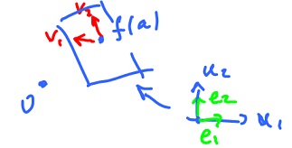
Generally, to find the image of an affine function, we use the fact that it's a hyperplane. We now need to know then the point a and the vectors that span the plane: $$v_1 = f'(a) e_1,$$
$$v_2 = f'(a) e_2,$$
where $e_1$ and $e_2$ are the basis of ${\bf R}^2$. Further, $f'(a)$ is a linear map and $v_1, v_2$ are linearly independent when $f$ is differentiable.
Review exercise. Find the spanning vectors of the plane: $$f_1'(a) = \left| \begin{array}{c} 0 & 0 \\ a+b & 0 \\ 0 & b \end{array} \right|$$
$$e_1 = ( 1, 0 )^T, e_2 = ( 0, 1 )^T.$$
$$\begin{array}{} v_1 &= f'(a) \cdot e_1 \\ &= \left| \begin{array}{c} 0 & 0 \\ a + b & 0 \\ 0 & b \end{array} \right| \left| \begin{array}{} 1 \\ 0 \end{array} \right| \\ &= \left| \begin{array}{c} 0 \\ a+b \\ 0 \end{array} \right| \end{array}$$
$$\begin{array}{} v_2 &= f'(a) \cdot e_2 \\ &= \left| \begin{array}{c} 0 & 0 \\ a+b & 0 \\ 0 & b \end{array} \right| \left| \begin{array}{} 0 \\ 1 \end{array} \right| \\ &= \left| \begin{array}{} 0 \\ 0 \\ b \end{array} \right| \end{array}$$
Answer: vertical plane, parallel to the $x_2,x_3$-plane.
As a review consider Find the point of the graph nearest to $0$.
Differentiation
Consider the norm:
$$f(x) = || x ||, x {\in} {\bf R}^n. $$
Then
$$f'(x) = \frac{1}{||x||} x^T.$$
Be careful how you write the best affine approximation now as the derivative has to be evaluated at the point of approximation, a, before it is substituted into the formula. So the answer is NOT
$$T(x) = \frac{1}{||x||} x^T ( x - a ) + || a ||$$
(it has to be affine, right?), but
$$T(x) = \frac{1}{|| a ||} a^T ( x - a ) + || a ||,$$
here
$( x - a )$ a vector (column matrix), and
Exercise. Find the derivatives of
$$|| x || x, e^{||x||}$$
Example.
$$h(x) = e^{||x||}, x {\in} {\bf R}^n.$$
Then $$h(x) = g( f(x) ),$$
$$g(y) = e^y, y = f(x) = || x ||,$$
$$g'(y) = e^y, f'(x) = \frac{1}{||x||} x^T.$$
With the Chain Rule, we obtain
$$h'(x) = g'(y) f'(y) = e^y \frac{1}{||x||} x^T = e^{||x||} \frac{1}{||x||} x^T,$$
(here $e^{||x||}$ and $\frac{1}{||x||}$ are numbers and $x^T$ a row vector).
Example. Let $$h: {\bf R}^n {\rightarrow} {\bf R}^2,$$
$$h(x) = ( || x ||, 3 || x || + 1 )^T,$$
then
$$h = g( f(x) ) {\rm \hspace{3pt} with \hspace{3pt}}$$
$$f: {\bf R}^n {\rightarrow} {\bf R}, f(x) = || x ||,$$
$$g: {\bf R} {\rightarrow} {\bf R}^2, g(y) = ( y, 3y + 1 )^T.$$
Then $$f'(x) = \frac{1}{||x||} x^T,$$
$$g'(y) = ( 1, 3 )^T,$$
$$\begin{array}{} h'(x) &= g'(y) f'(x) \\ &= ( 1, 3)^T \frac{1}{||x||} x^T \\ &= \frac{1}{||x||} \left| \begin{array}{} 1 \\ 3 \end{array} \right| ( x_1 ... x_n ) \\ &= \frac{1}{||x||} \left| \begin{array}{} x_1 & \ldots & x_n \\ 3x_1 & \ldots & 3x_n \end{array} \right| \end{array}$$
Theorem (Chain Rule). Suppose $h(x) = g( f(x) )$, where
$$f: {\bf R}^n {\rightarrow} {\bf R}^m, g: {\bf R}^m {\rightarrow} {\bf R}^q, h: {\bf R}^n {\rightarrow} {\bf R}^q. $$
Suppose further that
- $f$ is differentiable at $x = a$ and
- $g$ is differentiable at $y = f(a)$.
Then
- $h$ is differentiable at $x = a$ and
- $h'(a) = g'( f(a) ) f'(a)$.
Note: this is matrix multiplication.
Theorem (Sum Rule). Suppose
Then
$( f + g )'(a) = f'(a) + g'(a)$.
Theorem (Product Rule). Suppose
$k: {\bf R}^n {\rightarrow} {\bf R}$ is differentiable at $x = a$.
Then
$( kf )'(a) = f(a) k'(a) + k(a) f'(a)$.
Note that since
$k'(a)$ is of dimension $1 {\times} n$ (and hence $f(a) k'(a)$ is of dimension $m {\times} n$),
$k(a)$ is a scalar,
$f'(a)$ is of dimension $m {\times} n$ (and hence $k(a) f'(a)$ is of dimension $m {\times} n$),
Further keep in mind that here
- derivatives are matrices,
- functions are vectors.
Example. Let $h: {\bf R}^n {\rightarrow} {\bf R}^n$ with
$$h(x) = || x || x,$$
and $$k(x) = || x ||, $$
$$f(x) = x, x {\in} {\bf R}^n.$$
Then $$k'(x) = \frac{1}{||x||} x^T,$$
(If $f(x) = v_0 {\in} {\bf R}^n$, then $f'(x) = 0$, the zero matrix.)
Now $$h'(x) = x \cdot \frac{1}{||x||} x^T + || x || \cdot I,$$
where $|| x || \cdot I$ is a $n {\times} n$ matrix of the form
$$\left| \begin{array}{} ||x|| & \ldots & 0 \\ \vdots & \ddots & \vdots \\ 0 & \ldots & ||x|| \end{array} \right|$$
and $x x^T$ is a $n {\times} n$ matrix of the form
$$\left| \begin{array}{} x_1^2 & x_1x_2 & \ldots \\ x_1x_2 & \ldots & \ldots \\ \vdots & \ddots & \vdots \\ \ldots & \ldots & x_n^2 \end{array} \right|$$
Exercise. (1) $( || x || )' = \frac{1}{||x||} x^T, x {\in} {\bf R}^n$
(2) $( || x ||^2 )' = g'(y) f'(x) = 2y \frac{1}{||x||} x^T = 2 || x || \cdot \frac{1}{||x||} x^T = 2x^T$ [crossed out: $x {\neq} 0$ ]
$${\bf R}^n {\rightarrow} {\bf R}; y = f(x) = || x ||, g(y) = y^2, y {\in} {\bf R},$$
$$f'(x) = \frac{1}{||x||} x^T, g'(y) = 2y.$$
$$( || x ||^2 )'|_{x=0} = 0.$$
(3) With Product Rule: $({\bf R}^n {\rightarrow} {\bf R}^n)$ $$\begin{array}{} ( || x ||^2 x )' &= ( || x ||^2 )' x + || x ||^2 x' \\ &= 2 x^T x + || x ||^2 I \\ &= 2 x x^T + || x ||^2 I. \end{array}$$
Note: $( x^3 )' = 3 x^2.$
The Mean Value Theorem
Corollary 1. Let $f: {\bf R}^n {\rightarrow} {\bf R}^m$
Then $f$ is constant.
This is a "corollary" because it follows from the Mean Value Theorem below (the exact same way as it does in Calc 1).
Theorem (Mean Value Theorem). Let $[ a, b ] {\subset} D(h)$, where $h$ is differentiable on $( a, b )$ and $h$ is continuous on $[ a, b ]$. Then
Indeed, the condition implies that the gradient is zero, so all the partial derivatives $\frac{\partial f_j}{\partial x_i}$ are zero, hence by the MVT, every component function $h = f_j$ of $f$ is constant with respect to each of the variables. Hence it is constant and $f$ is constant too.
Another theorem that follows from the IVT is this.
Corollary 2. Let $f'(x) = g'(x)$ for all $x$ in an open subset $U$ of ${\bf R}^n$ and $f(a) = g(a)$. Then
In order to prove the Corollary, take $h = f - g$, then apply Corollary $1$.
Proof of the Chain Rule
Chain Rule: The derivative of the composition is equal to the composition of the derivatives (or product if we have matrices).
Let
$g: {\bf R}^m {\rightarrow} {\bf R}^q$ differentiable at $y = b = f(a).$
Then
and the derivative of the composition is equal to the composition of the derivatives.
By definition these three mean the existence of their best affine approximations (1) $T_f(x) = f(a) + f'(a) ( x - a)$,
(2) $T_g(y) = g(b) + g'(b) ( y - b ),$
Now we want to find what is the best affine approximation of the composition:
(3) $T_h(x) = h(a) + h'(a) ( x - a )$,
Idea: Prove that $T_g \circ T_f$ (satisfies (3)) is the best affine approximation of $h$.
(1) $\rightarrow$ Let $E_f(x) = \frac{f(x)-T_f(x)}{||x-a||}$,
Then $f(x) = T_f(x) + E_f(x) || x - a ||$.
(2) $\rightarrow$ Let $E_g(y) = \frac{g(y) - T_g(y)}{|| y - b ||},$
Then $g(y) = T_g(y) + E_g(y) || y - b ||$.
Consider
$$h(x) = g( f(x) ) = T_g( f(x) ) + E_g( f(x) ) || f(x) - b ||,$$
where
Then
$$\begin{array}{} h(x) &= T_g( T_f(x) + E_f(x) || x - a || ) + {\rm \hspace{3pt} small \hspace{3pt} term} \\ &= [ g(b) + g'(b) ( y - b ) ] ( T_f(x) + E_f(x) || x - a || ) + {\rm \hspace{3pt} small \hspace{3pt} term}. \end{array}$$
With
$$y = T_f(x) + E_f(x) || x - a ||$$
we get
$$\begin{array}{} h(x) &= g(b) + g'(b) ( T_f(x) + E_f(x) || x - a || - b ) + {\rm \hspace{3pt} small \hspace{3pt} term} \\ &= g(b) + g'(b) ( T_f(x) - b ) + g'(b) ( E_f(x) || x - a || ) + {\rm \hspace{3pt} small \hspace{3pt} term} \\ &= g(b) + g'(b) ( T_f(x) - b ) + {\rm \hspace{3pt} small \hspace{3pt} term} \end{array}$$
since
$g'(b) ( E_f(x) || x - a || ) {\rightarrow} 0$ as $x {\rightarrow} a$ because $g'(b)$ is linear.
Now
$$\begin{array}{} h(x) &= g(b) + g'(b) ( f(a) + f'(a) ( x - a ) - b ) + {\rm \hspace{3pt} small \hspace{3pt} terms} \\ &= g( f(a) ) + g'( f(a) ) ( f'(a) ( x - a ) ) + {\rm \hspace{3pt} small \hspace{3pt} terms} \\ &= h(a) + g'( f(a) ) f'(a) ( x - a ) + {\rm \hspace{3pt} small \hspace{3pt} terms}. \end{array}$$
Define
$$T_h(x) := h(a) + g'( f(a) ) f'(a) ( x - a ),$$
then $h(x) - T_h(x)$ is small in the sense that
So $T_h(x)$ is the best affine approximation, its linear part is the derivative of $h ( g'( f(a) ) \circ f'(a) {\rightarrow}$ Chain Rule ).
Parametrized hypersurfaces
Hypersurface in ${\bf R}^n$ is an $(n-1)$-dimensional manifold embedded in ${\bf R}^n$.
A parametric surface in ${\bf R}^3$ is the image of a function $f: {\bf R}^2 {\rightarrow} {\bf R}^3$ or
$$f: {\bf R}^2 {\supset} D(f) {\rightarrow} {\bf R}^3.$$
Not every image looks like a surface though. For example, let $f: {\bf R}^2 {\rightarrow} {\bf R}^3$.
(1) $f( x, y ) = ( 0, 0, 0 )$ for all $x, y$. $f'(a)$ $= 0$.
(2) $f( x, y ) = ( 0, 0, x )$ for all $x, y$.
$$f'(a) = \left| \begin{array}{} 0 & 0 \\ 0 & 0 \\ 1 & 0 \end{array} \right|$$
The image is a line, the $x_3$-axis.
(3) For the image to look "good", like a surface, we need
To understand why is suffices to look at $f$ that is linear...
Example. Let's parametrize the cylinder. The idea is to take the plane (the input space) and roll it into the cylinder (the image).
We want:
To guarantee that we define
$$f: \left\{ \begin{array}{} x_1 = f_1(x,y) & x{\rm -axis \hspace{3pt} only} \\ x_2 = f_2(x,y) & x{\rm -axis \hspace{3pt} only} \\ x_3 = f_3(x,y) & {\rm \hspace{3pt} with \hspace{3pt}} f_3(x,y)=y \end{array} \right. $$
So, $( x, y )$ on $y$-axis is $( 0, y )$,
$$x_3 = f_3( x, y ) = f_3( 0, y ) = y.$$
($y = 0$, $x$-axis, it is rolled into a circle):
So we want to parametrize the circle
$$f_1( x, y ) = {\rm sin \hspace{3pt}} x$$
$$f_2( x, y ) = {\rm cos \hspace{3pt}} x ({\rm multi-layered}),$$
$$f( x, y ) = ( {\rm sin \hspace{3pt}} x, {\rm cos \hspace{3pt}} x, y ).$$
Example. Parametrize
$$x_3 = x_1^2 + x_2^2.$$
Easy because one variable is express explicitly in terms of the other two. Define:
$$x_1 = f_1( x, y ) = x$$
$$x_2 = f_2( x, y ) = y$$
$$x_3 = f_3( x, y ) = x^2 + y^2.$$
The sphere would take some work:
$$x_1^2 + x_2^2 + x_3^2 = 1.$$
Level sets
Given $u = f(x)$ for $f: {\bf R}^n {\rightarrow} {\bf R}$, then for each $c {\in} {\bf R}$ the level set relative to $c$ of $f$ is
In other point these are points with the same altitude.
Is it always a curve?
Could be a point - if this is a local maximum or minimum.
Example. Let
$$z = x^2 + y^2,$$
paraboloid. The $0$-level curve for $c = 0$ is a point $( 0, 0 )$.
What would be a level set that is not a curve, but that isn't a maximum or a minimum?
Answer: A saddle point.
Ex. Let
$$z = x^2 - y^2,$$
the $0$-level set is
$x^2 = y^2$, or
i.e. two lines.
What do these two examples have in common? They both are critical points, i.e.
$$f'( a, b ) = 0,$$
so that the tangent plane is horizontal.
Theorem (Implicit Function Theorem). Let
$$f: {\bf R}^2 {\rightarrow} {\bf R}, f(a) = c, a {\in} {\bf R}^2, c {\in} {\bf R}.$$
Suppose
- $f$ is differentiable on an open disk $D$ around $a$, and that
- $f'$ is continuous on $D$.
Suppose further
$$f'(a) {\neq} 0. $$
Then the intersection of the $c$-level set with $D$ is a curve (i.e., it can be parametrized).
The name, Implicit Function Theorem, makes sense as an implicitly ($f(a) = c$) represented function can be represented explicitly.
Ex.
- Implicit: $x^2 + y^2 = 1$,
- Explicit:
$$\begin{array}{} y &= g(x) \\ &= \pm ( 1 - x^2 )^{\frac{1}{2}} \\ &= + ( 1 - x^2 )^{\frac{1}{2}} {\rm \hspace{3pt} if \hspace{3pt}} y > 0 \\ &= - ( 1 - x^2 )^{\frac{1}{2}} {\rm \hspace{3pt} if \hspace{3pt}} y < 0. \end{array}$$
How does the theorem apply here?
The theorem is easy to modify to get an analogue for parametric surfaces: If
$$f: {\bf R}^3 {\rightarrow} {\bf R}, f(a) = c, a {\in} {\bf R}^3, c {\in} {\bf R}$$
and $f$ is differentiable on an open ball $B$ around $a$, and $f'$ is continuous on $B$, and $f'(a) {\neq} 0$, then the intersection of the $c$-level set with $B$ is a surface.
Now, we have the theorem for curves in dimension $1$ and for surfaces in dimension $2$. The $n$ dim analogue is obvious.
Addendum.
is the tangent plane to the level surface at $( a, f(a) )$ in ${\bf R}^3$.
Ex.Consider the circle
$$x^2 + y^2 = 1.$$
Problem: Find the tangent line to the circle at the point $( \frac{\sqrt{2}}{2}, \frac{\sqrt{2}}{2} )$. The implicit differentiation yields
$$\frac{d}{dx} ( x^2 + y^2 ) = \frac{d}{dx} ( 1 ),$$
$$2x + 2y \frac{dy}{dx} = 0, y = y(x),$$
Ex. Consider
$$f( x, y, z ) = x^2 + xz - y^2 = 0$$
at $a = ( 1, 1, 0 )$. The surface is the $0$-level set of $f$,
$${\nabla}f = ( 2x + z, -2y, x ),$$
Solve
$$< ( 2, -2, 1 ), ( x, y, z ) - ( 1, 1, 0 ) > = 0$$
$$< ( 2, -2, 1 ), ( x - 1, y - 1, z ) > = 0$$
$$2( x - 1 ) - 2( y - 1 ) + z = 0.$$
For more see Parametric surfaces.


