Tutorial

Redirect to:

• Pixcavator help

This is a detailed overview of how to use Pixcavator. You may want to start with this quick tour instead or you may pick something related to your own field from our list of image analysis examples.

This article is to be replaced with a new one called Pixcavator help. It's not to be updated anymore...

Overview

Pixcavator is an image analysis program for scientists and researchers. It captures objects in the image by means of contours (outlines) and produces an Excel spreadsheet with those objects locations and measurements.

The processing goes through three main stages:

• Stage 1: automatic. A data structure is created that contains complete information about all possible segmentations of the image.
• Stage 2: semi-automatic. The user moves sliders corresponding to objects’ characteristics to instantly change their boundaries and choose the best segmentation. The output data is updated in real time.
• Stage 3: manual. The user can exclude noise and irrelevant details from the analysis by simply clicking on them.

Currently, Pixcavator has the following tabs.

• Analysis allows the user to load the image and start the analyze.
• Tools allows the user to manipulate the image using common image processing tools and special effects
• Output allows the user to view, explore and save the output data and the updated image.

Read about Pixcavator's system requirements.

Load an image and set up analysis

Start at the Analysis tab.

Select an image file from your computer by using the Choose image… button on the right. Most popular formats are supported: JPEG, BMP, PNG, GIF, TIFF.

The image will appear in the window on the left.

You can pan it using the left button of your mouse. The right button provides you with a magnification tool.

Note: when you open a new image, the previous analysis data is discarded.

Analysis of large images will take longer. The estimated processing time for gray scale images may be estimated by:

40 * width of the image * height of the image / 1000,000 seconds. 

This data is displayed on the right. Simpler images take less time, complex more. It will take about 25 seconds to process a gray scale 512×512 image. See Processing time.

If you are interested mainly in image analysis, smaller details within the image may be of relatively low interest. If this is the case, consider shrinking the image.

Use the slider marked with Shrink factor.

It is important to remember that both dimensions of the image are reduced. Therefore, if the slider is set at m, each of the two the dimensions of the image will be shrunk by m. As a result the processing time will be reduced by m*m.

Example. If you set the slider at 2, the processing time will be cut by a factor of 2*2=4.

For your convenience, this slider is preset so that the processing time is under 10 seconds. The use of this option is also appropriate for the initial analysis of a large image before you commit yourself to a long wait.

Keep in mind that once the image is shrunk, it is the new image that will be analyzed. Generally, this will not affect the number of objects detected as long as they are "large" and stay apart from each other. However, the sizes and locations of the objects will be displayed relative to the shrink coefficient.

Another way of thinking about shrinking the image is as reducing image resolution.

For more on this and examples of how to deal with shrinking and stretching, see Image scaling.

There is another way to improve the processing speed. Using the image processing tools (below) crop a small but important portion of the image and analyze it. This will remove the unwanted clutter in the image and will make the analysis more meaningful.

At this point you also choose the RGB channel you want to analyze.

Modify the image with image processing tools

Even if your interest is only in image analysis, you may want to try to modify the image with some image processing tools.

Go to the Tools tab. The image on the left is the original and the one on right will show the effects of these operations. You can enhance the original image before analyzing it or enhance the simplified image after analyzing it.

You can adjust the image’s Brightness, Contrast, Hue, and Saturation by using the sliders on the left. This may enhance the image and make it better suitable for analysis.

On the right, there is a drop down menu for Filters and effects.

• The most important tools for image analysis are at the top – Basic tools: Dilation and erosion, Crop, Subtract, Add border, Blur, Median filter, Noise, etc.

Some of these add imperfections to the image. They simulate real life effects and can be used to test the robustness of image analysis.

The rest of the items in this menu add artistic effects to the image.

For more see Pixcavator's image processing tools.

Analyze the image and view output

Process the image by pressing Run in the Analysis tab.

During this stage a data structure, called the topology graph, is created that contains complete information about all possible segmentations of the image.

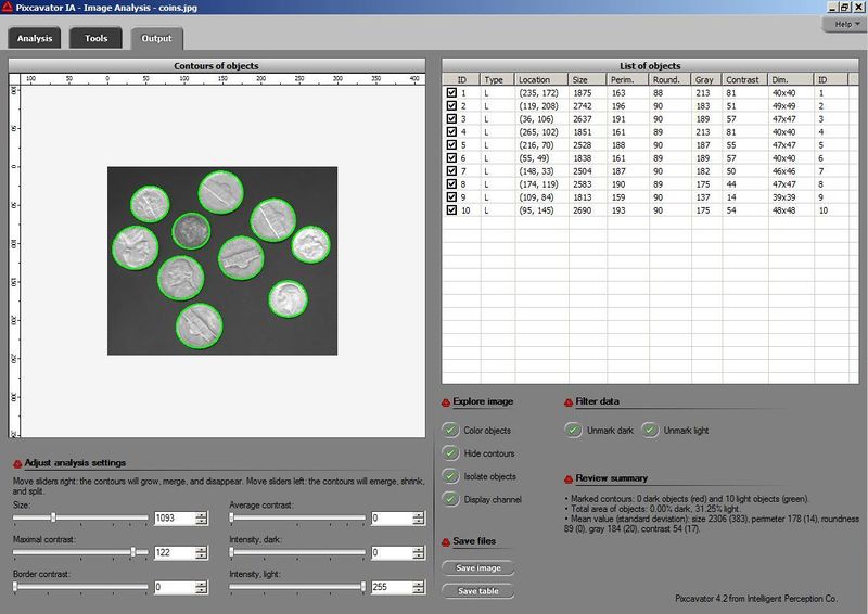
In the Output tab the analyzed image is now displayed on the left. Each object that has been detected is captured with a contour. Dark objects are outlined with red and light with green. To understand what they are exactly, read Boundaries in gray scale images. As before, you can pan with the left button of your mouse and magnify with the right button.

If you click within the image while holding Ctrl, the nearest object to your mouse will be marked or unmarked. If, in addition, you move the mouse, the objects close to the rectangle spanned this way will be marked or unmarked. As a result, the corresponding squares or contours will appear or disappear.

On the right, there is a table containing all objects in the image satisfying the current analysis settings. For each objects the following data is displayed:

• light or dark,
• location (coordinates of the centroid = the center of mass of the object as a lamina of uniform density),
• size (the number of pixels = area),
• perimeter,
• roundness (above 80 for circles, less for everything else),
• intensity (max/min level of gray),
• location of the center of mass (of the object as a lamina with density = gray level), -- not currently
• average contrast (saliency/size),
• thickness and length.

This table, combined with the settings, statistical summary etc, can be saved to hard disk in the form of a spreadsheet by pushing Save table.

For more see Pixcavator's output table.

Change analysis settings with sliders

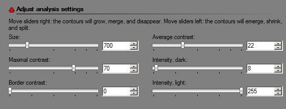
There are three sliders on the left that allow you to edit the analysis settings. The objects that fall below these thresholds will be ignored by the analysis procedure and not counted (to understand what we consider an object in an image read Objects in gray scale images).

To see how moving the sliders change the contours see this short clip.

First, choose a threshold for Size. For example, if you choose 100, every object containing less than 100 pixels will not captured or counted. The Size slider is set automatically depending on the size of the image.

Second, choose a threshold for Contrast. For example, if you choose 20, every object surrounded by an area with gray level that differs from that of the object by less than 20 will be ignored. There are 256 levels of gray.

This is how it works with these two sliders: the objects in the image are allowed to grow – from one level of gray to the next - up to the extent set by the slider (see Boundaries in gray scale images). For example, the object will grow until it’s both larger than say 100 pixels and has contrast above 20.

The third, Border contrast, slider is very different from the other two. Here, the object is allowed to expand – from one level of gray to the next - as long as its border moves less than a certain amount. Roughly, the expansion stops once the contour reaches a sharp edge. (To reproduce results you obtained with versions 3.0 and earlier, keep this value at 0.) Both this and the second slider consider the difference in intensity inside the object from that of the surrounding area. But, while the contrast slider considers the maximal difference throughout the object ("Max contrast"), the border contrast slider looks at the area just inside the contour. The result is: it detects sharp edges, i.e. the contours with the largest difference between what’s just inside and what’s just onside of it.

In version 4.2 three new sliders were introduced.

The fourth slider works similarly to the third but takes into account the average difference in intensity inside the object from that of the surrounding area. It’s called Average contrast.

The last two sliders simply threshold the image. For example, if you set Intensity, dark, to 100, the contours of dark objects displayed will have the intensity equal to exactly 100. If you set Intensity, light to 100, the contours of light objects will the intensity equal to exactly 155 (here 155=255-100). The last slider was set this way in order to ensure that contours grow as you move any of the six sliders from left to right. This is a very unsophisticated tool but it’s quite effective when the image lighting is uniform.

Keep in mind that if the analysis results are unsatisfactory, you don't have to start over! As you move the sliders, all data is re-computed very quickly, for images of reasonable size. You can experiment with the settings as the table and contours are updated almost instantly every time you move the sliders.

When you need to move a slider from A to B and if you stop along the way, the program starts to recompute the output. When the image is large or complicated, the recomputing might take seconds. To deal with this problem you may try not to stop as you drag the slider. In fact, even if you do stop, you are given 1/2 second before recomputing starts. Another way is to simply type the value you want in the window to the right of the slider.

Explore output image and data

Just like with any spreadsheet, if you click a column header, the rows in the table will be sorted from high to low or low to high with respect to the entries in this column.

To mark and unmark a row in the table, check and uncheck the square in the beginning of the row. If an object is marked or unmarked in the table on the right, a contour appears or disappears around it in the image on the left, and vice versa.

There are several headers on the right...

Explore image

You can erase everything outside the marked objects by pressing Isolate objects. See Background removal.

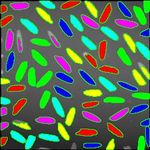
You can randomly color objects, marked only. See Coloring objects.

You can hide contours. To see the original image you used to have to go to the Analysis tab. Now you can flick it on and off to see what is hiding under the contours. The marking/unmarking of objects is unaffected.

You can Display channel that has been analyzed. For example if Red was selected in the Analysis tab, the red component of the image is displayed as a gray scale image. See RGB channels.

Filter data

There are only two buttons here currently – Unmark dark and Unmark light. These are toggle buttons so that you can choose to concentrate on only, say, light objects. You don't have to unmark dark every time you change the settings. See also Filtering output data.

Save files

You can save the displayed image - with all contours or squares, all marked, unmarked, or isolated objects – by pressing Save image. Finally, you can export the output table to Excel by pressing Save table.

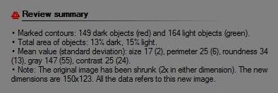
Review summary

The output table contains only the raw data about each object. Of course, if you save the data to Excel, you can get anything from it: average of all columns, histograms, etc. We thought that it would be nice to be able to preview some data: average values of size and contrast. The analysis summary includes the Mean values and Standard deviations of all the main characteristics of objects (marked only). To ensure accuracy, it is recommended that only images less then 2000x2000 are used with less than 1000 objects listed.

Pixcavator captures contours of all objects – light and dark - and displays all their measurements. If, however, there is just one object but with a few holes, it is important to see that this data gives you the area of what’s inside the contour. What you frequently need instead is the area of the object, which is

the area of what’s inside the contour - the areas of the holes.

A new feature is a step in that direction. Pixcavator now displays the two numbers above - the total area of dark and the total area of light – as percentages of the total size of the image (second row). So, to find the area of a dark object with light holes in it, one has to subtract these two numbers. (Caution: You have to make sure however that the holes are in the object not the background).

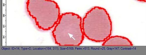
Hover over an object and view its data. It's displayed right under the image. That’s a new, convenient feature. You used to have to mark/unmark object in the image and then find the row in the table to see the object's measurements. That’s not a good idea if the table is a hundred rows long. Now you let the mouse hover over the object of your interest and the data from the table is displayed right beneath the image.

The next feature helps with image exploration. As you move the mouse around the analyzed image, the object you hover over is highlighted. The contour is shown blue and, if "Color objects" is selected, the whole object is colored. The data about it is displayed under the image as before.

Also, read Analysis strategy and Filtering output data.

Another exposition of this material is in the User Guide.

Read about real-life applications of Pixcavator under Examples, as well as Testing Pixcavator.