This site is being phased out.
Elementary PDEs
Contents
The PDE of heat propagation
To model heat propagation, imagine a grid of square rooms and the temperature of each room changes by a proportion of the average of the temperature of the four adjacent rooms. Its spreadsheet simulation is seen in the two images below; they are the initial state (a single initial hot spot) and the results (after $1,700$ iterations) for the temperature at the border fixed at $0$:
We will postpone the topic of heat propagation in higher dimensional spaces until later and concentrate on the $1$-dimensional case: the heat is contained in a row of rooms and each room exchanges the material with its two neighbors through its walls.
Suppose
- $a=AB$ is one of the rooms;
- $b,c$ are the two adjacent rooms, left and right;
- $A,B$ are the walls of $a$, left and right;
- $p=A^\star,q=B^\star$ are the two pipes from $a$, left and right.
What makes this different from ODEs is that the cochains will have two variables and two degrees -- with respect to location and with respect to time. The amount of heat $U=U(a,t)$ is simply a number assigned to each room $a$ which makes it a $1$-cochain. It also depends on time which makes it also a $0$-cochain.
A careful look reveals that to model heat transfer, we need to separately record the exchange of heat with each of the adjacent rooms.
The process we are to study obeys the following law of physics.
Newton's Law of Cooling: The rate of cooling of an object is proportional to the difference between its temperature and the ambient temperature.
This law is nothing but a version of the ODE of population growth and decay -- with respect to the exterior derivative $d_t$ over time. For each cell there are two adjacent cells and two temperature differences, $d_x$, to be taken into account. The result is a partial differential equation (PDE).
Notation:
- $d_t$ is the exterior derivative with respect to time; and
- $d_x$ is the exterior derivative with respect to location. $\\$
Either is simply the difference in ${\mathbb R}$.
The conservation of energy in cell $a$ gives us the following. The change of the amount of the heat in room $a$ over the increment of time is equal to $$d_t U(a)=-\bigg( \text{ sum of the outflow } F \text{ across the walls of } a\bigg).$$ The outflow gives the amount of flow across a node (from the room to its neighbor) per unit of time. It is a dual $1$-cochain. Specifically, the flow is positive at $A$ if it is from left to right and the opposite for $B$; then: $$d_t U(a)=-\big( F^\star(A)-F^\star(B) \big) = F^\star(A)-F^\star(B),$$ which is the exterior derivative of this $0$-cochain.
Now, we need to express $F$ in terms of $U$. The flow $F(A^\star)=F^\star(A)$ through wall $A$ of room $a$ is proportional to the difference of the amounts of heat in $a$ and the other room adjacent to $A$. So, $$F^\star(A) = - k(A)d_x(U^\star)(A^\star).$$ Here, $k(A) \ge 0$ represents the permeability of the wall $A$ at a given time. Specifically, $$\begin{array}{lll} F^\star(A) &= - k(A) \big( U(a) - U(b) \big),\\ F^\star(B) &= - k(B) \big( U(c) - U(a) \big). \end{array}$$
Naturally, the walls form the boundary $\partial a$ of $a$. Therefore, we can rewrite: $$d_t U(a)= -F^\star(\partial a)$$ or, by the Stokes Theorem, $$d_t U(a) = -(d_x F^\star)(a).$$
The result of the substitution is a PDE of second degree called the heat equation of cochains: $$d_t U = d_x \big( kd_x U^\star \big)^\star.$$ Specifically, we have: $$d_t U(a) = \Big(- k(A) \big( U(a) - U(b)\big)\Big) - \Big(- k(B) \big( U(c) - U(a)\big)\Big). $$ The right-hand side becomes the increment in the recursive formula for the simulation: $$U(a, t+1):= U(a,t) + \Big[- k(a) \big( U(a) - U(a-1)\big) + k(a+1) \big( U(a+1) - U(a)\big)\Big].$$ The initial state is shown below:
Note: When the domain isn't the whole space, the pipes at the border of the region have to be removed. In the spreadsheet, we use boundary conditions to substitute for the missing data.
The result after $1,500$ iterations is shown next:
One can clearly see how the density becomes uniform eventually -- but not across an impenetrable wall ($k(A_5)=0$).
Link to file: Spreadsheets.
Exercise. For an infinite sequence of rooms, what is the limit of $U$ as $t\to \infty$?
Exercise. Create a simulation for a circular sequence of rooms. What is the limit state?
Exercise. Generalize the formula to the case when the permeability of walls depends on the direction.
Transfer depends on geometry
We now consider the general case of edges/rooms of arbitrary size. Then what determines the dynamics of the heat transfer isn't the amount of heat $U(a)$ in room $a$ but its temperature, i.e., the average amount of heat: $U(a)/|a|$.
In summary, the amount of heat exchanged between two rooms is proportional to:
- the temperature difference,
- the permeability of the wall (dually: the conductance of the pipe),
- the area of the wall that separates them (dually: the cross section of the pipe), and
- inversely, to the distance between the centers of mass of the rooms (dually: the length of the pipe).
Let's split the data into three categories:
- the adjacency of rooms (and the pipes) is the topology,
- the areas of the walls (and the lengths of the pipes) is the geometry, and
- the properties of the material of the walls (and the pipes) is the physics. $\\$
They are given by, respectively:
- the domain ${\mathbb R}$,
- the lengths of the edges of ${\mathbb R}$ and ${\mathbb R}^\star$, and
- the $0$-cochain $k$ over ${\mathbb R}$.
In addition to the above list, the amount of material exchanged between two rooms is also proportional to the length of the current time interval $|t|$. Then our PDE takes the form: $$d_tUq^{-1}=(kU_x)_x|t|,$$ with both sides $(n,0)$-cochains. Consider the first derivative with respect to time: $$U_{t}:=U'=\star d_t U=\tfrac{1}{|t|}d_tU.$$
The heat equation is: $$U_t q^{-1}= (kU_x)_x.$$
The abbreviated version is below. $$\begin{array}{|c|} \hline \\ \quad U_t = (kU_x)_x \quad \\ \\ \hline \end{array}$$
Second, it's the lengths of the $1$-cells dual to the endpoints of $a=AB$: $$\frac{1}{|A^\star|},\frac{1}{|B^\star|}.$$ The denominators are the lengths of the pipes.
Conclusion: The amount of heat exchanged by a primal $1$-cell $a$ with its neighbor $a'$ is
- directly proportional to the difference of density in $a$ and $a'$, and
- inversely proportional to the length of the pipe that leaves $a$ for $a'$.
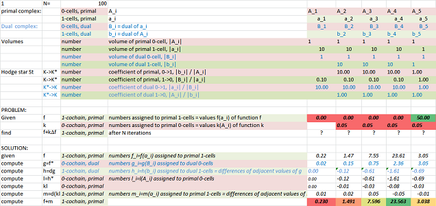
To confirm these ideas, we run a spreadsheet simulation below:
With a single initial spike in the middle, we see that the amounts of material in the smaller cells on the right: $$|a_5|=|a_6|=|a_7|=|a_8|=|a_9|=1,$$ quickly become uniform, while the larger ones on the left: $$|a_1|=|a_2|=|a_3|=|a_4|=10,$$ develop slower.
Link to file: Spreadsheets.
Exercise. Find the speed of propagation of the material in a uniform grid as a function of the length of the cell.
Exercise. Suppose we have two rods made of two different kinds of metal soldered together side by side. The cells will expand at two different rates when heated. Model the change of its geometry and illustrate with a spreadsheet. Hint: Assign a thickness to both.
The PDE of wave propagation
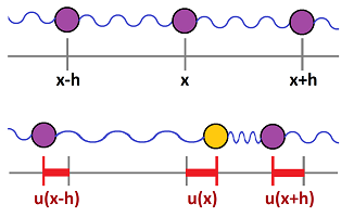
Previously, we studied the motion of an object attached to a wall by a (mass-less) spring. Imagine this time a string of objects connected by springs:
Just as above, we will provide the mathematics to describe the following three parts of the setup:
- the topology of the cell complex $L$ of the objects and springs,
- the geometry given to that complex such as the lengths of the springs, and
- the physics represented by the parameters of the system such as those of the objects and springs.
Let $u(t,x)$ be the function that measures the displacement from the equilibrium of the object associated with position $x$ at time $t$ (we will suppress $t$). It is an algebraic quantity: $$u=u(t,x)\in R.$$ As such, it can represent quantities of any nature that may have nothing to do with a system of objects and springs; it could be an oscillating string:
Here, the particles of the string are vertically displaced while waves propagate horizontally (or we can see the pressure or stress vary in a solid medium producing sound).
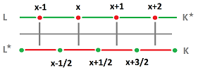
First, we consider the spatial variable, $x\in {\bf Z}$. We think of the array -- at rest -- as the standard $1$-dimensional cubical complex $L={\mathbb R}_x$. The complex may be given a geometry: each object has a (possibly variable) distance $h=\Delta x$ to its neighbor and the distance between the centers of the springs has length $\Delta x^\star$. We think of $u$ as a cochain of degree $0$ -- with respect to $x$.
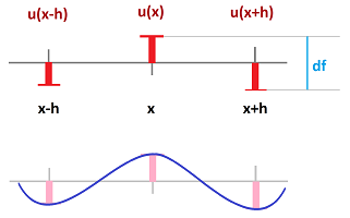
According to Hooke's law, the force exerted by the spring is $$F_{Hooke} = -k df,$$ where $df\in R$ is the displacement of the end of the spring from its equilibrium state and the constant, stiffness, $k\in R$ reflects the physical properties of the spring. If this is the spring that connects locations $x$ and $x+1$, its displacement is the difference of the displacements of the two objects. In other words, we have: $$df=u(x+1) - u(x).$$ Therefore, the force of this spring is $$H_{x,x+1} = k \Big[ u(x+1) - u(x) \Big].$$ Since $k$ can be location-dependent, it is a $1$-cochain over $L$.
Now, let $H$ be the force that acted on the object located at $x$. There are two Hooke's forces acting on this object from the two adjacent springs: $H_{x,x-1}$ and $H_{x,x+1}$. Therefore, we have: $$\begin{array}{lll} H &= H_{x,x-1} &+ H_{x,x+1} \\ &= k \Big[ u(x-1) - u(x) \Big] &+ k\Big[ u(x+1) - u(x) \Big]\\ &=-(kd_xu)[x-1,x]&+(kd_xu)[x,x+1]. \end{array}$$
Next, we investigate what this means in terms of the Hodge duality. These are the duality relations of the cells involved: $$\begin{array}{llll} &[x-1,x]^\star &= \{x-1/2 \},\\ &[x,x+1]^\star &= \{x+1/2 \},\\ &\{x\}^\star &= [x-1/2,x+1/2]. \end{array}$$ Then the computation is straight-forward: $$\begin{array}{llll} H&= (kd_xu)\Big([x+1,x]-[x,x-1]\Big)\\ &= (kd_xu)\Big(\{x+1/2 \}^\star -\{x-1/2 \}^\star\Big)\\ &=(\star kd_xu)\Big( \{x+1/2\}-\{x-1/2\}\Big)\\ &= d_x(\star kd_xu)\Big( [x-1/2,x+1/2] \Big)\\ &=d_x(\star kd_xu)(x^\star)\\ &=\star d_x\star kd_xu(x)\\ &=\star d_xk^\star \star d_xu(x)\\ &=(k^\star u_x)_x(x). \end{array}$$
Second, we consider the temporal variable, $t\in {\bf Z}$. We think of time as the standard $1$-dimensional cubical complex ${\mathbb R}_t$. The complex is also given a geometry. It is natural to assume that the geometry has no curvature, but each increment of time may have a different duration (and, possibly, $\Delta t \ne \Delta t^\star$). We think of $u$ as a cochain of degree $0$ with respect to $t$.
Now suppose that each object has mass $m$. Then, by the Second Newton's Law, the total force is $$F=m \cdot a,$$ where $a$ is the acceleration. It is the second derivative with respect to time, i.e., this $0$-cochain: $$a=u_{tt}:=\star d_t \star d_t u . $$ The mass $m$ is a $0$-cochain too and so is $F$. Note that the stiffness $k$ is also a $0$-cochain with respect to time.
Now, with these two forces being equal, we have derived the wave equation of cochains: $$\begin{array}{|c|} \hline \\ \quad m u_{tt} = (k^\star u_x)_x. \quad \\ \\ \hline \end{array}$$
If $k$ and $m$ are constant cochains (and $R$ is a field), the wave equation takes a familiar shape: $$u_{tt}=\tfrac{k}{m}u_{xx}.$$
Simulating wave propagation with a spreadsheet
Now we will derive the recurrence relations.
First, we assume that the geometry of the time is “flat”: $\Delta t =\Delta t^\star$. Then the left-hand side of our equation is $$m d_{tt} u = m\frac{u(x,t+1)-2u(x,t)+u(x,t-1)}{(\Delta t)^2}.$$ For the right-hand side, we can use the original expression: $$ \star d_x \star k d_xu = k \Big[ u(x-1) - u(x) \Big] + k\Big[ u(x+1) - u(x) \Big].$$
Second, we assume that $k$ and $m$ are constant. Then just solve for $u(x,t+1)$: $$\begin{array}{ll} u(x,t+1) &= 2u(x,t) - u(x,t-1) + \alpha\Big(u(x+1,t)-2u(x,t)+u(x-1,t)\Big), \end{array}$$ where $$\alpha :=(\Delta t)^2 \frac{k}{m}.$$
To visualize the formula, we arrange the terms in a table: $$\begin{array}{l|cccccc} & x-1 & x & x+1\\ \hline t+1 & & u(x,t+1) \\ t &=\alpha u(x-1,t) & +2(1-\alpha)u(t,x) & +\alpha u(x+1,t)\\ t-1 & & -u(x,t-1) \end{array}$$ Even though the right-hand side is the same, the table is different from that of the (dual) diffusion equation. The presence of the second derivative with respect to time makes it necessary to look two steps back, not just one. That's why we have two initial conditions.
We suppose, for simplicity, that $\alpha=1$.
Example. Choosing the simplified settings allows us to easily solve the following initial value problem: $$\begin{array}{lll} u_{tt}=u_{xx};\\ u(x,t)=\begin{cases} 1 &\text{ if } t=0,x=1;\\ 0 &\text{ if } t=0,x\ne 1;\\ 1 &\text{ if } t=1,x=2;\\ 0 &\text{ if } t=1,x\ne 2. \end{cases} \end{array}$$ Initially, the wave has a single bump and then the bump moves one step from left to right. The negative values of $x$ are ignored.
Now, setting $k=1$ makes the middle term in the table disappear. Then every new term is computed by taking an alternating sum of the three terms above, as shown below: $$\begin{array}{l|cccccccc} t \backslash x& 1 & 2 & 3 & 4 & 5 & 6 & 7 & ..\\ \hline 0 & 1 & 0 & 0 & 0 & 0 & [0] & 0 & ..\\ 1 & 0 & 1 & 0 & 0 & [0] & 0 & [0] & ..\\ \hline 2 & 0 & 0 & 1 & 0 & 0 & (0) & 0 & ..\\ 3 & 0 & 0 & 0 & 1 & 0 & 0 & 0 & ..\\ 4 & 0 & 0 & 0 & 0 & 1 & 0 & 0 & ..\\ 5 & 0 & 0 & 0 & 0 & 0 & 1 & 0 & ..\\ .. & .. & .. & .. & .. & .. & .. & .. & .. \end{array}$$ We can see that the wave is a single bump running from left to right at speed $1$:
$\square$
Exercise. (a) Solve the two-sided version of the above IVP. (b) Set up and solve an IVP with $2$ bumps, $n$ bumps.
Exercise. Implement a spreadsheet simulation for the case of non-constant $m$. Hint: you will need two buffers.
The recurrence formula for dimension $1$ wave equation and constant $k$ and $m$ is: $$\begin{array}{ll} u(x,t+1) &= 2u(x,t) - u(x,t-1) + \alpha\Big[u(x+1,t)-2u(x,t)+u(x-1,t)\Big], \end{array}$$ with $$\alpha :=(\Delta t)^2 \frac{k}{m}.$$ We put these terms in a table to be implemented as a spreadsheet: $$\begin{array}{l|cccccc} & x-1 & x & x+1\\ \hline t-1 & & -u(x,t-1) \\ t &=\alpha u(x-1,t) & +2(1-\alpha)u(t,x) & +\alpha u(x+1,t)\\ t+1 & & u(x,t+1) \end{array}$$
The simplest way to implement this dynamics with a spreadsheet is to use the first two rows for the initial conditions and then add one row for every moment of time. The Excel formula is: $$\texttt{ = R1C5*R[-1]C[-1] + 2*(1-R1C5)*R[-1]C + R1C5*R[-1]C[1] - R[-2]C}$$ Here cell $\texttt{R1C5}$ contains the value of $\alpha$.
Link to file: Spreadsheets.
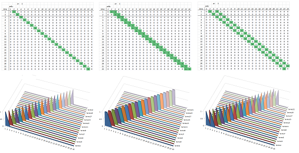
Example. The simplest propagation pattern is given by $\alpha=1$. Below we show the propagation of a single bump, a two-cell bump, and two bumps:
$\square$
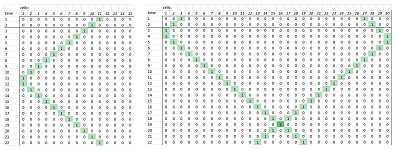
Exercise. Modify the spreadsheet to introduce walls into the picture:
Exercise. Modify the spreadsheet to accommodate non-constant data by adding the following, consecutively: (a) the stiffness $k$ (as shown below), (b) the masses $m$, (c) the time intervals $|\Delta t|$.


