Differential calculus of parametric curves

Parametric curves

Recall that the Tangent Problem asks for a tangent line to a curve at a given point. It has been solved for the graphs of numerical functions in Chapter 7. However, most of the curves in real life can't be represented as graphs. We have to look at parametric curves. The examples are familiar.

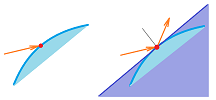
Example. In which direction a radar signal will bounce off a plane when the surface of the plane is curved?

In what direction will light bounce off a curved mirror?

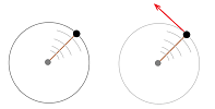
In what direction would a rock released from a sling go?

And so on. $\square$

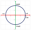
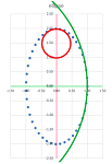
Example. Let's confirm that the sound originating from one focus of an elliptical room will bounce off the wall to pass through the other focus.

This way one can listen to a conversation at the other focus even if there are obstacles between them. $\square$

Now, we study functions. They all have a single variable input and a single variable output. What varies is the nature of these two variables.

A parametric curve is such a function: $$F:t\mapsto F(t).$$

• The single independent variable is a real number, $t$.
• The single dependent variable is multi-dimensional, a point or a vector in ${\bf R}^n$.

For example for $n=2$, we may have $$F: t\mapsto X=(f(t),\ g(t)),$$ or $$F: t\mapsto OX=<f(t),\ g(t)>.$$ As we know, the former point, $X$, is the end of the latter vector, $OX$. In either case, this is just a combination of two function of the same independent variable.

The go-to metaphor for parametric curves is motion:

• $t$ is thought of as time,
• $(f(t),g(t))$ is thought of as the position in space at time $t$.

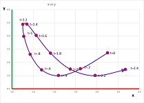
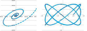
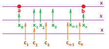
We plot each $(x,y)$ and label each with the corresponding values of $t$:

These values of $t$ may come as the nodes of a partition of an interval $[a,b]$ or run through the whole interval.

Example (straight line). Linear motion is represented as follows:

• $F(t) = V \cdot t$, a motion along a vector $V$ (constant speed) from the origin;
• $F(t) = V \cdot t + B$, same but with $B$ the starting location;
• $F(t) = - V \cdot t = V \cdot (-t)$, backward;
• $F(t) = V \cdot (t^2)$, accelerated.

$\square$

Example (circle). The distance to some point remains the same, say, $1$, and the implicit equation is $$x^2+y^2=1.$$

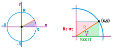
The “simple” circular motion happens when the angular velocity is constant: the object turns the same angle per unit of time: $$F(t) = <\cos t,\ \sin t>.$$ We substitute $x=\cos t$ and $y=\sin t$ into the equation and use the Pythagorean Theorem to prove that this is indeed the unit circle: $$x^2+y^2=(\cos t)^2+(\sin t)^2=1.$$

There are other ways to travel around a circle of course. Circling $0$ but moving backward: $$F(t) = <\cos (-t),\ \sin (-t)>;$$ circling $0$ but along radius $r$: $$F(t) = r \cdot <\cos t,\ \sin t>;$$ circling point $(p,q)$: $$F(t) = (p,q) + r \cdot <\cos t,\ \sin t>.$$ For the accelerated motion, just change how fast the time goes: $$F(t) = <\cos t^2,\ \sin t^2>.$$ $\square$

Example (ellipse). The implicit equation of the ellipse is $$\frac{x^2}{a^2}+\frac{y^2}{b^2}=1,$$ for some non-zero constant numbers $a,b$. Now, the “simple” elliptic motion is similar to circular motion happens when the angular velocity is constant but the distance varies. $$F(t) = <a\cos t,\ b\sin t>.$$ We substitute $x=a\cos t$ and $y=b\sin t$ into the equation and use the Pythagorean Theorem to prove that this is indeed the ellipse: $$\frac{x^2}{a^2}+\frac{y^2}{b^2}=\frac{(a\cos t)^2}{a^2}+\frac{(b\sin t)^2}{b^2}=\cos^2 t+\sin ^2t=1.$$

Other ways to travel around an ellipse are shown below. Circling $0$ but moving backward: $$F(t) = <a\cos (-t),\ b\sin (-t)>;$$ circling point $(p,q)$: $$F(t) = (p,q) + r \cdot <a\cos t,\ b\sin t>.$$ $\square$

Curves -- given as graphs or implicitly -- can be parametrized. It is as if we need to get the shape of the road and achieve that by driving along the road while recording the time and the location.

Definition. A parametric curve $X=X(t)$ is called a parametrization of a curve $C$ in ${\bf R}^n$ when the path of $X$ coincide with the curve $C$.

In the above examples we showed a variety of way to parametrize lines, circles, and ellipses.

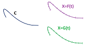
Theorem. If the function t=g(s) is one-to-one and onto, then the two parametric curves $$X=F(t) \text{ and } X=F(g(s))$$ are parametrizations of the same curve.

Definition. The parametrization of the ellipse that uses the angle of the line from the origin as the parameter is called the standard parametrization of the ellipse.

The graphs of functions are especially easy to parametrize.

Theorem. The parametric curve $x=t,\ y=f(t)$ is a parametrization of the graph of $y=f(x)$.

It is as if we are moving east at a constant speed...

Definition. For $n=2$, we call the parametric curve $$\begin{cases} x=t,\\ y=f(t), \end{cases}$$ the standard parametrization of the graph $y=f(x)$.

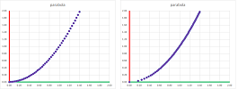
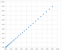
Example (parabola). The standard parametrization of the parabola $y=x^2$ is (left): $$F(t) = (t, t^2).$$

Meanwhile this parametrization of the parabola $x=\sqrt{y}$ is different (right): $$G(t) = (\sqrt{t}, t).$$ $\square$

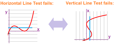
Conversely, we can sometimes represent the path of a plane parametric curve as the graph of a function. This function is

• $y=f(x)$ if the path satisfies the Horizontal Line Test, or
• $x=g(y)$ if the path satisfies the Vertical Line Test.

The circle fails both! However, it can be “de-parametrized” piece-by-piece (top-bottom or left-right halves). This would be a challenging task for more complex curves:

Representing a plane curve as a parametric curve from the beginning is a strongly preferred approach.

Algebraically, we try to eliminate the parameter by solving for $t$ followed by substitution: $$\begin{cases} x=t^3\\y=\sin t\end{cases}\ \Longrightarrow\ t=\sqrt[3]{x}\ \Longrightarrow\ y=\sin\left(\sqrt[3]{x}\right).$$ The scheme works only when one of the component functions is one-to-one.

The motion may also be in the $3$-dimensional space:

• $t$ is thought of as time,
• $(f(t),g(t),h(t))$ is the position in space at time $t$.

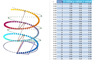
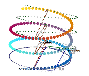
We plot each $(x,y,z)$ and label each with the corresponding values of $t$.

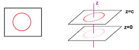
Example (circle in space). $$F(t) = (\cos t, \sin t, c).$$

In a plane $x=c$ parallel to the $xy$-plane. $\square$

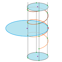
Example (helix). An ascending spiral is when the rotation in the horizontal plane is combined with a vertical ascend: $$F(t) = (\cos t, \sin t, t)$$

$\square$

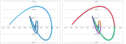
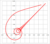
Exercise. Suggest a parametric representation for the curve below:

We will revisit every issue about functions we considered in Parts I and II as they apply to parametric curves.

But first we consider the issue that lies at the heart of calculus: the rate of change. We take another look at the location-velocity-acceleration connection.

Limits

We have always assumed that to get from point $A$ to point $B$, we have to visit every location between $A$ and $B$.

If there is a jump in the path of the parametric curve, it can't represent motion! Then the question becomes the one about the integrity of the path: is there a break or a cut? Thus, we want to understand what is happening to $x=f(t),\ y=g(t)$ when $t$ is in the vicinity of a chosen input value $t=s$.

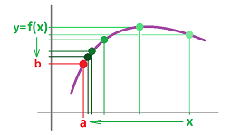
This is how we handled the problem in dimension $1$. For the curve represented by the graph of $y=f(x)$ we say that $f(x)$ approached $b$ as $x$ approaches $a$: $$f(x)\to b \text{ as } x\to a.$$

The picture can also be described as follows:

• $x$ is approaching $a$, and
• $y$ is approaching $b$.

This coordinate-wise thinking isn't good enough for us anymore and that is why we rephrase one more time:

• a point $(x,y)$ on the curve is approaching point $(a,b)$.

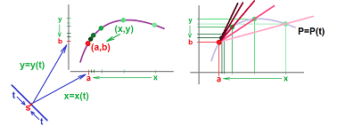
This way to express the idea of limit is fully applicable to parametric curves! The difference this time is that $y$ doesn't depend on $x$ anymore; instead, $x=x(t)$ and $y=y(t)$ depend on $t$. This is what we have: $$(x,y)\to (a,b) \text{ as } t\to s,$$ for some real number $s$.

More generally, we a parametric curve is a function defined on a closed interval in ${\bf R}$ with values in ${\bf R}^n$ (treated as either points or vectors): $$X(t)\to A \text{ as } t\to s.$$ Only the former part needs to be explained.

How do we know that points $X(t)$ are approaching another point $A$? This means that $X(t)$ is getting closer and closer to $A$ or, more precisely, the distance from $X(t)$ is getting smaller and smaller and, in fact, approaching zero.

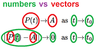
Definition. The limit of a parametric curve $X=X(t)$ in ${\bf R}^n$ at $t=s$ is defined to be such a point $A$ in ${\bf R}^n$ that $$d(X(t),A)\to 0\text{ as } t\to s.$$ For vectors, the analogous definition is: $$||X(t)-A||\to 0\text{ as } t\to s.$$

In either case, we use the notation: $$\lim_{t\to s} X(t)=A,$$ or $$X(t)\to A\text{ as }t\to s.$$

Note how vectors converge in both the magnitude and direction.

We have thus defined a new concept, the limit of a parametric curve, by relying entirely on something familiar: the limit of the usual, numerical functions! Alternatively, we can take a direct route below. We mimic the theory of limits of functions and concentrate on a sequence converging to the point.

Example. Suppose we would like to study this parametric curve around the point $t=0$: $$x=\cos x,\ y=x^2.$$ The reciprocal sequence is an appropriate choice: $$t_n=\frac{1}{n}\to 0.$$ Recall that the composition of any function and a sequence gives us a new sequence... $\square$

Example. Consider the graph of the function $\operatorname{sign}$ around $0$. Its standard parametrization is $x=t,\ y=\operatorname{sign}(t)$.

We try $t_n=-1/n$ and $s_n=1/n$: $$\lim_{n\to \infty} \operatorname{sign}(-1/n)=-1 \text{ but } \lim_{n\to \infty} \operatorname{sign}(1/n)=1,$$ as we approach $0$ from one direction at a time. The limits don't match! $\square$

The alternative definition is in the following theorem.

Theorem. The limit of a parametric curve $X=X(t)$ in ${\bf R}^n$ at $t=s$ is the limit of these sequences of point in ${\bf R}^n$ $$\lim_{n\to \infty} X(t_n)$$ considered for all sequences $\{t_n\}$ within the domain of $X$ excluding $s$ that converge to $s$, $$s\ne t_n\to s \text{ as } n\to \infty,$$ when all these limits exist and are equal to each other. Otherwise, the limit does not exist.

This is what happens for $n=2$:

Let's concentrate on parametric curves as vector-valued function. This is the definition of the limit:

Since the outputs of these functions are vectors, all the algebraic operations available for vectors are also possible for functions (parametric curves):

• vector addition,
• scalar multiplication (the scalar might itself depend on $t$!), and
• the dot product (the outcome is a scalar function!).

Under these operations, the limits are preserved.

Let's consider them one by one.

Theorem (Sum Rule). If the limits at $t=s$ of parametric curves $X=F(t)$ and $X=G(t)$ exist then so does that of their sum, $X=F(t) \pm G(t)$, and the limit of the sum is equal to the sum of the limits: $$\lim_{t\to s} \big(F(t) + G(t)\big) = \lim_{t\to s} F(t) + \lim_{t\to s} G(x).$$

Proof. We can prove the result by using the above theorem; as follows: for any sequence $t\to s$, we have by SR for sequences: $$\lim_{t\to s} (F(t) + G(t)) = \lim_{n\to \infty} (F(t_n)+G(t_n)) = \lim_{n\to \infty} F(t_n)+\lim_{n\to \infty} G(t_n).$$ Alternatively, we use the definition. If $A$ and $B$ are the two limits, we consider and manipulate the following expression: $$\begin{array}{lccccl} ||(F(t)+G(t))-(A+B)||&=&||(F(t)-A)&+&(G(t)-B)||&\text{...re-arranging terms}\\ &\le& ||(F(t)-A)||&+&||(G(t)-B)||&\text{...using the Triangle Inequality}\\ &&\downarrow & & \downarrow &\text{...taking the limits}\\ &=&0 &+&0&\text{...zeros by the definition}\\ &=&0. \end{array}$$ By the definition, we conclude that $F(t)+G(t)\to A+B$. $\blacksquare$

Theorem (Constant Multiple Rule). If the limit at $t=s$ of a parametric curve $X=F(t)$ exists then so does that of its multiple, $X=c F(t)$, and the limit of the multiple is equal to the multiple of the limit: $$\lim_{t\to s} c F(t) = c \cdot \lim_{t\to s} F(t).$$

Proof. We can prove the result by using the above theorem just as in the last proof: for any sequence $t\to s$, we have by CMR for sequences: $$\lim_{t\to s} \big(cF(t)\big) = \lim_{n\to \infty} \big(cF(t_n)\big) = c\lim_{n\to \infty} F(t_n).$$ Alternatively, we use the definition. If $A$ is the limit, we consider and manipulate the following expression: $$\begin{array}{lcccl} ||\big(cF(t)\big)-\big(cA\big)||&=&||c\cdot &(F(t)-A)||&\text{...factoring}\\ &=& |c|\cdot &||(F(t)-A)||&\text{...using the Homogeneity}\\ &&||&\downarrow &\text{...taking the limit}\\ &=&|c|\cdot&0 &\text{...zero by the definition}\\ &=&0. \end{array}$$ By the definition, we conclude that $cF(t)\to cA$. $\blacksquare$

What if the multiple isn't constant?

Theorem (Variable Multiple Rule). If the limits at $t=s$ of a parametric curve $X=F(t)$ and a function $r=c(t)$ exist then so does that of their product, $X=c(t) \cdot F(t)$, and the limit of the product is equal to the product of the limits: $$\lim_{t\to s} \big( c(t) \cdot F(t) \big) = \big(\lim_{t\to s} c(t)\big)\cdot\big( \lim_{t\to s} F(t)\big).$$

Exercise. Modify the proof of the Constant Multiple Rule to prove the last theorem.

Theorem (Dot Product Rule). If the limits at $t=s$ of parametric curves $X=F(t)$ and $X=G(t)$ exist then so does that of their dot product, $r=F(t) \cdot G(t)$, and the limit of the dot product is equal to the dot product of the limits: $$\lim_{t\to s} \big(F(t) \cdot G(t)\big) = \big(\lim_{t\to s} F(t)\big)\cdot\big( \lim_{t\to s} G(t)\big).$$

This is a summary of how limits behave with respect to the usual algebraic operations.

Theorem (Algebra of Limits). Suppose $F(t)\to A$ and $G(x)\to B$ as $t\to s$. Then $$\begin{array}{|ll|ll|} \hline \text{SR: }& F(t)+G(t)\to A+B & \text{CMR: }& c F(t)\to cA& \text{ for any real }c\\ \text{DPR: }& F(t)\cdot G(t)\to A\cdot B&\text{VMR: }& c(t) F(t)\to bA& \text{ when }c(t)\to b \\ \hline \end{array}$$

Now the asymptotic behavior of parametric curves. All graphs are parametric curves, so the latter exhibit just as many types of large-scale behavior as the former.

We will however mention here only the patterns that are coordinate-independent. They are

• convergence to a point,
• divergence to infinity, and
• periodicity.

The first one is defined just as the common limit but instead of $t$ approaching some $s$, $t\to s$, we have $t$ approaching infinity, $t\to\infty$.

Definition. We say that a parametric curve $X=X(t)$ approaches point $A$ as $t\to\pm\infty$ if $$||X(t)-A||\to 0 \text{ as } t\to \pm\infty .$$ Then we use the notation: $$X(t) \to A \text{ as }t\to \pm\infty,$$ or $$\lim_{t\to\pm\infty}X(t)=A.$$

There are infinitely many directions in ${\bf R}^n,\ n>1,$ and that's the reason we consider only one infinity: the graph is simply running away from $0$.

Definition. We say that a parametric curve $X=X(t)$ goes to infinity if $$||X(t_n)||\to \infty,$$ for any sequence $t_n\to \pm\infty$ as $n\to \infty$. Then we use the notation: $$X(t) \to \infty \text{ as }t\to \pm\infty,$$ or $$\lim_{t\to\pm\infty}X(t)=\infty.$$

Example. From the familiar facts: $$\lim_{t \to -\infty} e^{t} = 0, \quad \lim_{t \to +\infty} e^{t} = +\infty,$$ we deduce that $$(t,e^t)\to\infty \text{ as } t\to\pm\infty.$$

$\square$

Example (Newton's Law of Gravity). We have already seen examples of some of these behaviors exhibited by a planet under the effect of gravity. They may be bounded or unbounded. Which one we are to observe depends on the initial conditions. Let's make the connection more precise.

$\square$

Continuity

A numerical function $y=f(x)$ is called continuous at point $x=a$ if $$\lim_{x\to a}f(x)=f(a).$$

Thus, the limits of continuous functions can be found by substitution.

We approach the issue of continuity of parametric curves in an identical fashion.

Definition. A parametric curve $X=X(t)$ is called continuous at $t=s$ if $$\lim_{t\to s}X(t)=X(s).$$

Example. Examples of continuity and discontinuity come from Chapter 6.

$\square$

Just as before, we can interpret continuity as just another algebraic rule of limits!

Theorem (Substitution Rule). If a parametric curve $X=X(t)$ is continuous at $t=s$ then $$\lim_{t\to s}X(t)=X(s).$$

A generalization of this rule is related to compositions.

Recall that the definition of limit of $X=X(t)$ at $t=s$ can be re-written as an implication:

• if $t$ is approaching $s$, then $X(t)$ is approaching $A$,

or, $$t\to s \ \Longrightarrow\ X=X(t)\to A.$$

Suppose we have a parametric curve $X$ in ${\bf R}^n$. An example of its composition with a function $z$ of $n$ variables was considered in Chapter 16: $$(z\circ X)(t)=z(X(t)).$$ As continuity of functions of several variables hasn't been treated yet, we postpone this example until Chapter 18 and instead look at the composition of $X$ with a numerical function $t=t(u)$ (on the other end): $$(X\circ t)(u)=X(t(u)).$$ Thus we have two functions processing three variables: $$u\mapsto t\mapsto X.$$ Furthermore, let's look at the limit of the composition function at some $v$: $$u\to v \ \Longrightarrow\ X=(X\circ t)(u)\to A,$$ if this $A$ exists. We break this into two. First: $$u\to v \ \Longrightarrow\ t=t(u)\to s.$$ Second, let's suppose that $X$ is continuous at this $t=s$. Then, $$t\to s \ \Longrightarrow\ X=X(t)\to X(s).$$ Together: $$u\to v \ \Longrightarrow\ t=t(u)\to s \ \Longrightarrow\ X=X(t)\to X(s).$$

Theorem (Composition Rule). Suppose $t=t(u)$ is a numerical function with: $$\lim_{u\to v}t(u)=s.$$ Suppose a parametric curve $X=X(t)$ is continuous at $t=s$. Then, $$\lim_{u\to v}(X\circ t)(u)=X(s).$$

This is a shortened version: $$\lim_{u\to v}X(t(u))=X\left( \lim_{u\to v}t(u) \right).$$ It reveals how a continuous function can be pulled out of a limit. In other words, the limit is, again, computed by substitution.

We now use the algebraic properties of limits to show how continuity is preserved under these operations.

Theorem (Continuity and Algebra). Suppose parametric curves $F$ and $G$ are continuous at $t=s$. Then so are the following:

• 1. (SR) the parametric curve $F\pm G$,
• 2. (CMR) the parametric curve $c\cdot F$, for any real number $c$,
• 3. (VMR) the parametric curve $c\cdot F$, for any continuous numerical function $c$, and
• 4. (DPR) the numerical function $F \cdot G$.

Some theorems about the behavior of continuous numerical functions have analogues for parametric curves.

First, in the multidimensional spaces there are no “larger” or “smaller” points or vectors. This is why we can't compare functions (or their limits) as easily as $f(x)<g(x)$ anymore. No comparison theorems then. For the same reason we can't easily squeeze a parametric curve between two other parametric curves. However, we can squeeze a parametric curve with a numerical function used to estimate the distance to another parametric curve. For dimension $n=2$, this is a narrowing strip:

For dimension $n=3$, it's a funnel.

Theorem (Squeeze Theorem). Suppose we have first: $$d(P(t),Q(t)) \leq h(t) ,$$ for all $t$ within some open interval from $t=s$; second: $$\lim_{t\to s} Q(t) = A;$$ and third: $$\lim_{t\to s} h(t) = 0.$$ Then $$\lim_{t\to s} P(t) = A.$$

Proof. The third condition guarantees that $$d(P(t),Q(t)) \to 0.$$ $\blacksquare$

For the vector-valued functions, the first condition becomes: $$||P(t)-Q(t)|| \leq h(t).$$

The definition of continuity is purely local: only the behavior of the function in the, no matter how small, vicinity of the point matters. What can we say about its global behavior?

Definition. A parametric curve $P=P(t)$ is called continuous on interval $I$ if it is continuous at every $s$ in $I$.

Definition. A parametric curve $X=X(t)$ is called bounded on an interval $[a,b]$ if there is such a real number $m$ that $$||X(t)|| \le m$$ for all $t$ in $[a,b]$.

In other words, the image of the function is within the sphere of radius $m$.

Theorem (Boundedness). A continuous on a closed bounded interval parametric curve is bounded on the interval.

Proof. The proof repeats the one for the $1$-dimensional case. Suppose, to the contrary, that $X$ is unbounded on interval $[a,b]$. Then there is a sequence $\{t_n\}$ in $[a,b]$ such that $X(t_n)$ is unbounded. Then, by the Bolzano-Weierstrass Theorem, sequence $\{t_n\}$ has a convergent subsequence $\{u_k\}$: $$u_k \to u.$$ This point belong to $[a,b]$! From the continuity, it follows that $$X(u_k) \to X(u) \text{ or } ||X(u_k) - X(u)||\to 0.$$ This contradicts the fact that $\{||X(u_k)||\}$ is a subsequence of a sequence that diverges to infinity. $\blacksquare$

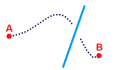
Our understanding of continuity of numerical functions has been as the property of having no gaps in their graphs. The Intermediate Value Theorem says also that there are no gaps in the ranges either. What about parametric curve? It's path should have no gaps. In other words, to get to the other side of the river we have to cross it!

This idea is more precisely expressed by the following.

Theorem (Intermediate Value Theorem). Suppose a parametric curve $X=X(t)$ on the plane is defined and is continuous on interval $[a,b]$. Suppose also that there is a line $L$ such that $X(a)$ and $X(b)$ lie on the different sides of $L$. Then there is a $d$ in $[a,b]$ such that $X(d)$ lies on $L$.

Exercise. Explain the meaning of “lie on the different sides of”.

This theorem motivates introducing the following important concept.

Definition. A subset $Q$ of ${\bf R}^n$ is called path-connected if any two points in $Q$ can be connected by a path, i.e., if $A$ and $B$ are two points in $Q$ then there is such a continuous parametric curve $X=F(t)$ defined on $[a,b]$ that $F(a)=A$ and $F(b)=B$.

Then the theorem tells us that the plane with a line removed, i.e., ${\bf R}^2\backslash L$ is not path-connected. The plane is, the circle too, a point but not two, a line, a sphere but not two, etc.

Next, once again, there are no “larger” or “smaller” points or vectors. This is why we can't speak of maximum and minimum points.

Theorem (Extreme Value Theorem). A continuous parametric curve on a bounded closed interval has a point of maximal distance from the origin, i.e., if $X=X(t)$ is continuous on $[a,b]$, then there is $c$ in $[a,b]$ such that $$||X(c)||\ge ||X(t)||,$$ for all $t$ in $[a,b]$.

Proof. It follows from the Bolzano-Weierstrass Theorem. $\blacksquare$

The coordinate-wise treatment for parametric curve follows from that for sequences presented in Chapter 16.

Theorem (Coordinate-wise convergence). As $t\to s$, we have $$X(t)\to A,$$ or $$X(t)=(p_1(t),\ p_2(t),\ ...,\ p_n(t))\to A=(a_1,\ a_2,\ ...,\ a_n),$$ if and only if $$p_1(t)\to a_1,\ p_2(t)\to a_2,\ ...,\ p_n(t)\to a_n.$$

Example. We compute: $$\begin{array}{lll} \lim_{t\to \pi/2}(\cos t,\ \sin t)&=\left( \lim_{t\to \pi/2}\cos t,\ \lim_{t\to \pi/2} \sin t \right)\\ &=(\cos \pi/2,\ \sin \pi/2)\\ &=(1,0), \end{array}$$ because $\sin t$ and $\cos t$ are continuous. $\square$

This theorem also makes it easy to prove the algebraic properties of limits of parametric curves from those for numerical functions. For example, the Dot Product Rule is proven below: $$\begin{array}{llll} \lim_{t\to s}\big( <x,y>\cdot <u,v> \big)&=\lim_{t\to s}(xu+yv)\\ &=\lim_{t\to s}(xu)+\lim_{t\to s}(yv)\\ &=\lim_{t\to s}x\cdot \lim_{t\to s}u+\lim_{t\to s}y\cdot \lim_{t\to s}v\\ &=<\lim_{t\to s}x,\ \lim_{t\to s}y>\cdot <\lim_{t\to s}u,\ \lim_{t\to s}v>. \end{array}$$

Now continuity. At $t=s$, suppose a parametric curve $$X(t)=(x(t),\ y(t),\ z(t))$$ is continuous at $t=s$. This is equivalent to the following, as $t\to s$, we have $$X(t)\to X(s)\ \Longleftrightarrow\ x(t)\to x(s),\ y(t)\to y(s),\ z(t)\to z(s) .$$ The latter is equivalent to the three component functions $x(t),y(t),z(t)$ being continuous at $t=s$.

Theorem (Coordinate-wise continuity). A parametric curve, $$X(t)=(p_1(t),\ ...,\ p_n(t)),$$ is continuous at $t=s$ if and only if all its component functions, $p_1(t),\ ...,\ p_n(t)$, are continuous at $t=s$.

Example. Is the circle a continuous curve? Yes, because the two functions in its parametrization $\cos t$, $\sin t$ are continuous. $\square$

Location - velocity - acceleration

We continue with some “pre-limit” calculus; we will revisit the location - velocity - acceleration issue in the context of parametric curves; the motion is on the plane.

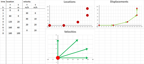
Suppose we drove around while paying attention both to the clock and to the mileposts. The result is this simple table with five columns: $$\begin{array}{|l|c|c|c|c|c|} \text{time (hours): }&0&2&4&6&8\\ \hline \text{location (miles): }&(0,0)&(60,0)&(120,20)&(160,60)&(160,100) \end{array}$$ So, we drove east and then north.

What was the velocity over these four periods of time? We estimate it with the familiar difference quotient: $$\text{average velocity}=\frac{\text{change of location}}{\text{change of time}},$$ except this time the numerator, and the average velocity itself, is a vector. These are the computations: $$\begin{array}{|l|cccccc|} \text{time (hours): }&0&2&4&6&8\\ \hline \text{location (miles): }&(0,0)&(60,0)&(120,20)&(160,60)&(160,100)\\ \hline \text{velocity (m/h): }&\tfrac{(60,0)-(0,0)}{2-0}=&<30,0>&&&\\ \text{velocity (m/h): }&&\tfrac{(120,20)-(60,0)}{4-2}=&<30,10>&&\\ \text{velocity (m/h): }&&&\tfrac{(160,60)-(120,20)}{6-4}=&<20,20>&\\ \text{velocity (m/h): }&&&&\tfrac{(160,100)-(160,60)}{8-6}=&<0,20>\\ \end{array}$$ The four computed values are the average velocities over the following intervals of time: $[0,2]$, $[2,4]$, $[4,6]$, and $[6,8]$, respectively. This is, of course, a partition. The summary is in this table: $$\begin{array}{|l|c|c|c|c|c|} \text{time intervals (hours): }&[0,2]& [2,4]&[4,6]&[6,8]\\ \hline \text{velocity (m/h): }&<30,0>&<30,10>&<20,20>&<0,20> \end{array}$$ Alternatively, we may choose to assign the four values to the middle points of these intervals, as the secondary nodes of the partition, as follows: $$\begin{array}{|l|c|c|c|c|c|} \text{time (hours): }&1&3&5&7\\ \hline \text{velocity (m/h): }&<30,0>&<30,10>&<20,20>&<0,20> \end{array}$$ This amount to simply choosing different secondary nodes in this partition of the interval.

This is the summary of what we have found:

We also compute the acceleration. Just as we used the “difference quotient” formula to find the velocity from the location, we now use it to find the acceleration from the velocity, as vectors: $$\text{average acceleration}=\frac{\text{change of velocity}}{\text{change of time}}.$$ We apply this formula to three periods of time. These are the computations: $$\begin{array}{|l|cccccc|} \text{time intervals (hours): }&[0,2]& [2,4]&[4,6]&[6,8]\\ \text{time (hours): }&1&3&5&7\\ \hline \text{velocity (miles/hour): }&<30,0>&<30,10>&<20,20>&<0,20>\\ \hline \text{acceleration (m/h/h): }&\tfrac{<30,10>-<30,0>}{3-1}=&<0,5>\\ \text{acceleration (m/h/h): }&&\tfrac{<20,20>-<30,10>}{5-3}=&<-5,5>\\ \text{acceleration (m/h/h): }&&&\tfrac{<0,20>-<20,20>}{7-5}=&<-10,0> \end{array}$$ The three computed values are the average accelerations over the following intervals of time: $[0,4]$, $[2,6]$, and $[4,8]$, respectively. This is the result: $$\begin{array}{|l|c|c|c|} \text{time intervals (hours): }&[0,4]&[2,6]&[4,8]\\ \hline \text{acceleration (m/h/h): }&<0,5>&<-5,5>&<-10,0> \end{array}$$ Alternatively, we may choose to assign the three values to the middle points of these intervals, as follows: $$\begin{array}{|l|c|c|c|} \text{time (hours): }&2&4&6\\ \hline \text{acceleration (m/h/h): }&<0,5>&<-5,5>&<-10,0> \end{array}$$

This is the summary of what we have found:

Next we reverse the problem: the acceleration is known and the velocity and the location are to be found.

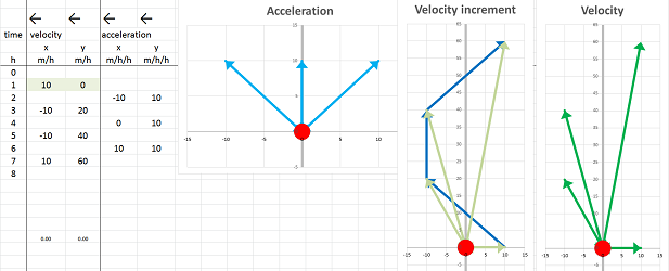
Suppose we start our motion at the initial location $(0,0)$ miles with an initial velocity $<10,0>$ miles per hour and proceed with the acceleration given below: $$\begin{array}{|l|c|c|c|} \text{time intervals (hours): }&[0,4]&[2,6]&[4,8]\\ \hline \text{acceleration (m/h/h): }&<-10,10>&<0,10>&<10,10> \end{array}$$ We now apply the same formulas as the one we used when the motion was described by a numerical function (or two): $$\text{next velocity } =\text{ current velocity }+\text{ acceleration }\cdot \text{ time increment},$$ except this time these quantities, except for time, are vectors.

We choose the time increment to be $2$. These are the computations: $$\begin{array}{|l|cccccc|} \text{time (hours): }&[0,2]&[2,4]&[4,6]&[6,8]\\ \hline \text{acceleration (m/h/h): }&<-10,10>&<0,10>&<10,10>\\ \hline \text{velocity (m/h): }&<10,0>\\ \text{velocity (m/h): }&+2<-10,10>=&<-10,20>&&\\ \text{velocity (m/h): }&&+2<0,10>=&<-10,40>&\\ \text{velocity (m/h): }&&&+2<10,10>=&<10,60>&\\ \end{array}$$

The four computed values are the average velocities over the following intervals of time: $$\begin{array}{|l|c|c|c|c|c|} \text{time intervals (hours): }&[0,2]&[2,4]&[4,6]&[6,8]\\ \hline \text{velocity (m/h): }&<10,0>&<-10,20>&<-10,40>&<10,60> \end{array}$$

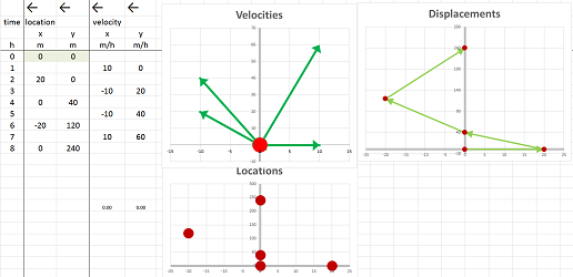
We compute the position next using the same, vector, formula: $$\text{next position } =\text{ current position}+\text{ velocity }\cdot \text{ time increment},$$ These are the results: $$\begin{array}{|l|cccccc|} \text{time (hours): }&0&2&4&6&8\\ \hline \text{velocity (m/h): }&<10,0>&<-10,20>&<-10,40>&<10,60>\\ \hline \text{position (m): }&(0,0)\\ \text{position (m): }&+2<10,0>=&(20,0)&&\\ \text{position (m): }&&+2<-10,20>=&(0,40)&\\ \text{position (m): }&&&+2<-10,40>=&(-20,120)&\\ \text{position (m): }&&&&+2<10,60>=&(0,240)&\\ \end{array}$$ This is the path: $$\begin{array}{|l|c|c|c|c|c|} \text{time (hours): }&0&2&4&6&8\\ \hline \text{location (miles): }&(0,0)&(20,0)&(0,40)&(-20,120)&(0,240) \end{array}$$

In summary, we have this collection of sequences for each of the dimensions of the space:

• $t_n$ for the time,
• $p_n$ for the position,
• $v_n$ for the velocity, and
• $a_n$ for the acceleration.

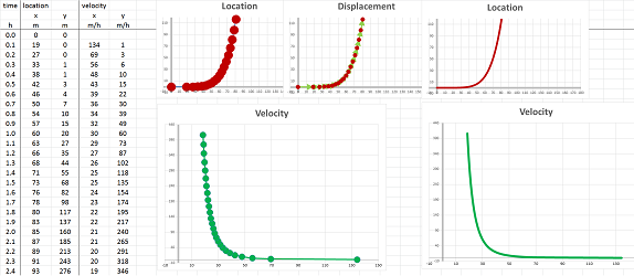
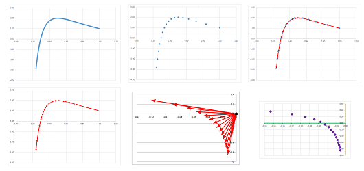
They are connected by these recursive formulas for each component: $$v_{n+1}=\frac{p_{n+1}-p_n}{t_{n+1}-t_n} \text{ and } a_{n+1}=\frac{v_{n+1}-v_n}{t_{n+1}-t_n},$$ or, for the inverse problem,, $$v_{n+1}=v_n+a_{n+1}(t_{n+1}-t_n) \text{ and } p_{n+1}=p_n+v_{n+1}(t_{n+1}-t_n).$$ With more data, the vectors of the velocities and the accelerations are used to trace out curves. For example, this is what computation of the velocity from location looks like:

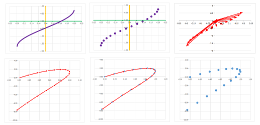
Note that the velocity column has one fewer data point and the acceleration one fewer yet. However, when zoomed out, the graphs look like actual continuous curves and give an impression that the three functions have the same domain.

The change and the rate of change: the difference and the difference quotient

We would like to construct the secant or tangent lines of a parametric curve at all points at the same time:

The result will be a function.

Suppose we know only two values of a function: $$F(a)=A\text{ and }F(b)=B,$$ with $a\ne b$. Then, what can we say about its rate of change? It is the change of $X$ with respect to the change of $t$. The former is the difference of $f$, denoted by: $$\Delta f=B-A=F(b)-F(a).$$ The latter is the increment of $t$, denoted by: $$\Delta t=b-a.$$ Their ratio is the rate of change of $F$, which we will call the difference quotient of $F$, given by: $$\frac{\Delta F}{\Delta t}=\frac{F(b)-F(a)}{b-a}.$$

Let's review the construction of a augmented partition $X$ of an interval $[a,b]$. We place the primary nodes (or simply nodes) on the interval: $$ a=t_{0}\le t_{1}\le t_{2}\le ... \le t_{n-1}\le t_{n}=b,$$ producing $n$ smaller intervals of possibly different lengths: $$ [t_{0},t_{1}],\ [t_{1},t_{2}],\ ... ,\ [t_{n-1},t_{n}],$$ with $t_0=a,\ t_n=b$. The lengths of the intervals are the increments of $t$: $$\Delta t_i = t_i-t_{i-1},\ i=1,2,...,n.$$ We are also given the secondary nodes of the partition: $$ c_{1} \text{ in } [t_{0},t_{1}], \ c_{2} \text{ in } [t_{1},t_{2}],\ ... ,\ c_{n} \text{ in } [t_{n-1},t_{n}].$$

Thus an augmented partition is simply a combination of points: $$ a=t_{0}\le c_1\le t_{1}\le c_2\le t_{2}\le ... \le t_{n-1}\le c_n\le t_{n}=b.$$ In the example in the last section we had a similar construction:

• the intervals of the partition were equal in length, and
• the secondary nodes were placed at the end of each interval.

Furthermore, we utilize the secondary nodes as the inputs of the new function:

Suppose $X=F(t)$ is defined at the nodes $t_k,\ k=0,1,2,...,n$, of the partition.

Definition. The difference of $F$ is defined at the secondary nodes of the partition by: $$\Delta F\, (c_{k})=F(t_{k})-F(t_{k-1}),\ k=1,2,...,n.$$

Definition. The difference quotient of $F$ is defined at the secondary nodes of the partition by: $$\frac{\Delta F}{\Delta t}(c_{k})=\frac{F(t_{k})-F(t_{k-1})}{t_k-t_{k-1}}=\frac{\Delta F(c_{k})}{\Delta t_k},\ k=1,2,...,n.$$

Note that when secondary nodes aren't provided, we can think of the intervals themselves as the inputs of the difference (and the difference quotient): $c_{k}=[t_{k-1},t_{k}]$. It is then a $1$-form, the difference of a $0$-form $F$.

When the context is clear, we use the simplified notation without the subscripts: $$\Delta F\, (c) \text{ and } \frac{\Delta F}{\Delta t}(c).$$

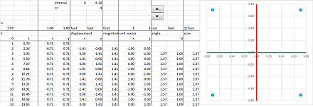
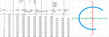
Example. Let's find the difference quotient of the circle parametrized the usual way: $$X(t)=(\cos t,\ \sin t).$$ We use the Trigonometric Formulas for the difference quotient from Chapter 7. Suppose we have a mid-point partition for the interval, say, $[-\pi/2,\pi/2]$, in the $t$-axis:

• the nodes are $x=a,a+h,...$ and
• the secondary nodes are $c=a+h/2,...$.

Then the difference quotients of $\sin x$ and $\cos x$ are given by at $c$: $$\begin{array}{lll} \frac{\Delta }{\Delta x}(\sin x)=\frac{ \sin (h/2)}{h/2}\cdot&\cos c;& \frac{\Delta }{\Delta x}(\cos x)=-\frac{ \sin (h/2)}{h/2}\cdot&\sin c.\\ \end{array}$$ Therefore, we can compute coordinate-wise: $$\frac{\Delta X}{\Delta t}(c)=\bigg<-\frac{ \sin (h/2)}{h/2}\cdot\sin c,\ \frac{ \sin (h/2)}{h/2}\cdot\cos c\bigg>=\frac{ \sin (h/2)}{h/2}<-\sin c,\ \cos c>.$$ $\square$

The instantaneous rate of change: derivative

Let's review a few examples of why we study derivatives. The problems we face are familiar but this time they are treated with parametric curves!

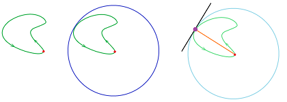
Example. Light bounces off a curved mirror as if off a straight mirror that is tangent to the mirror at the point of contact.

$\square$

Example. The head lights of a car traveling on a curvy road point in the tangent direction to the road at that particular location.

$\square$

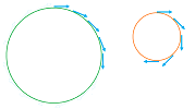
Example. The direction a rock will go when released from a sling is tangent to the circle at the point of release.

$\square$

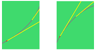
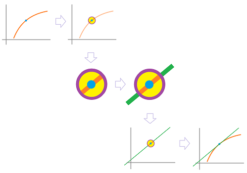
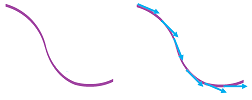
Recall how we zoom in on the point and realize that it is virtually a straight line, the tangent line at $A$:

The method of constructing the tangent is to build a sequence of lines that cut through the graph. Each passes through two points, $A$ and some $B$ with $A\ne B$.

What is the difference this time? First we aren't looking for the slope of this line anymore but rather its direction vector.

Next, with a numerical function, the change of $x$ brings about the change of $y$ and their ratio is the average rate of change and, after the limit, the derivative of the function. With a parametric curve, it is the same for the two components: the change of $t$ brings about the change of $x$ and $y$ and these two ratios are the average rates of change and, after the limit, the two components of the vector of the derivative of the curve.

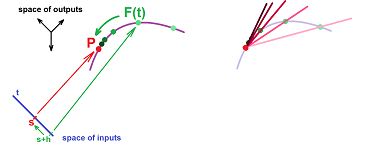
The coordinate-free interpretation is: the change of $t$ brings about the change of point $X$ and this ratio (of a vector and a number) is the average rate of change and, after the limit, the vector of the derivative of the curve. This description applies to any dimension:

• $t$ changes from $s$ to $s+h$, and
• $X$ changes from $X=F(s)$ to $Q=F(s+h)$.

Here, $h$ is the increment of the input. It is often denoted by $h=\Delta t$ while the increment of the output is denoted by $\Delta X$. Then,

• the change of $t$ is number $h$, and
• the change of $X$ is vector $XQ$.

In terms of motion, these are the increment of time and the displacement. We conclude that

• the rate of change of $X$ with respect to $t$ is vector

$$\frac{1}{h}XQ\text{ or } \frac{\Delta X}{\Delta t}.$$ It is also known as the difference quotient or, in the context of motion, the average velocity.

Warning: when units are involved, as in the case of motion, the vector of the rate of change lies in a space different from the original (and that of the vector of the change of $X$).

The next step is to make $h$ smaller and smaller. This will make the displacement vector shorter and shorter approaching vector $0$ (unless the parametric curve is discontinuous!) but not necessarily the vector of the rate of change. The latter might have a limit!

Definition. Suppose a parametric curve $X=F(t)$ is defined on an open interval $I$ that contains $t=s$. Then the derivative of $F$ at $t=s$ is the following limit, if exists, denoted by: $$F'(s)=\lim_{h\to 0}\frac{1}{h}(F(s+h)-F(s)),$$ or $$\frac{dF}{dt}(s)=\lim_{h\to 0}\frac{1}{h}(F(s+h)-F(s)).$$ When this limit exists, the parametric curve $F$ is called differentiable at $t=s$.

Note that the definition is the same if we choose to think of our parametric curve as vector-valued. The result is a new vector-valued function, i.e., a new parametric curve!

Example. Let's test the definition in a familiar territory. For any two vectors $A$ and $B$, we have $$\begin{array}{lll} (At+B)'&=\lim_{h\to 0}\frac{1}{h}\bigg[(A(t+h)+B)-(At+B)\bigg]\\ &=\lim_{h\to 0}\frac{1}{h}\big[A(t+h)-At\big]\\ &=\lim_{h\to 0}\frac{1}{h}\big[Ah\big]\\ &=\lim_{h\to 0}A\\ &=A. \end{array}$$ Then, the derivative of a parametric curve of a line is its direction vector! $\square$

More generally, we have a familiar formula for “vector polynomials”.

Theorem. For any vectors $A_m,\ A_{m-1},...,\ A_1,\ A_0$ in ${\bf R}^n$, we have $$\bigg(A_mt^m+A_{m-1}t^{m-1}+...+A_1t+A_0\bigg)'=A_mt^{m-1}+A_{m-1}t^{m-2}+...+A_1.$$

Exercise. Prove the theorem.

When the function is discontinuous, there is a gap in the path. Then the displacements might not converge to $0$! In that case, the limit above can't exist.

Theorem. Every differentiable parametric curve is also continuous.

Exercise. Prove the theorem.

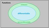
Example. Examples of differentiable and non-differentiable functions come from Chapter 7.

If the graph of the absolute value function is parametrized the usual way, $x=t,\ y=|t|$, the resulting parametric curve is continuous but not differentiable. $\square$

Exercise. (a) Prove the last statement. (b) Find a differentiable parametrization of $y=|x|$.

Computing derivatives

The derivative is a limit and we can use facts about limits we have discussed. We compute derivatives of parametric curves component-wise.

Example (circular motion). Let's consider the circle under standard parametrization: $$F(t)=<\cos t,\ \sin t>.$$ We can think of this as if an object is moving around the circle -- at a constant angular velocity.

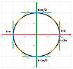
We compute its derivative according to its definition: $$\begin{array}{llrlll} F'(t)&=\lim_{h\to 0}\frac{1}{h}&(F(t+h)&-F(t))&\\ &=\lim_{h\to 0}\frac{1}{h}&\bigg(<\cos (t+h),\ \sin (t+h)>&-<\cos t,\ \sin t>\bigg)&\text{...substitute}\\ &=\lim_{h\to 0}\frac{1}{h}&\bigg<\cos (t+h)-\cos t,& \sin (t+h)-\sin t\bigg>&\text{...vector addition}\\ &=\lim_{h\to 0}&\bigg<\frac{1}{h}(\cos (t+h)-\cos t),& \frac{1}{h}(\sin (t+h)-\sin t)\bigg>&\text{...scalar multiplication}\\ &=\lim_{h\to 0}&\bigg<\frac{1}{h}(\cos (t+h)-\cos t),& \frac{1}{h}(\sin (t+h)-\sin t)\bigg>&\text{...limit component-wise}\\ &=&\bigg<\lim_{h\to 0}\frac{1}{h}(\cos (t+h)-\cos t), &\lim_{h\to 0}\frac{1}{h}(\sin (t+h)-\sin t)\bigg>&\text{...the derivatives}\\ &=&<(\cos t)',& (\sin t)'>&\text{...of the two functions}\\ &=&<-\sin t,& \cos t>&\text{}\\ \end{array}$$ Let's confirm the results: $$\begin{array}{lll|lll} F'(0)&=<0,1>& \text{vertical} &F'(\pi/4)&=\bigg<-\dfrac{\sqrt{2}}{2},\ \dfrac{\sqrt{2}}{2}\bigg>& \text{diagonal}\\ F'(\pi/2)&=<-1,0>& \text{horizontal}&F'(3\pi/4)&=\bigg<-\dfrac{\sqrt{2}}{2},\ -\dfrac{\sqrt{2}}{2}\bigg>& \text{diagonal}\\ ...&&&... \end{array}$$ These are the direction vectors of the tangent lines:

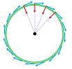
Further examination reveals that the vector $F'(t)$ of the velocity rotates as $t$ increases. Specifically, $F'(t)$ is perpendicular to $F(t)$: $$F(t)\cdot F'(t)=<\cos t,\ \sin t>\cdot <-\sin t,\ \cos t> =-\cos t\sin t+\sin t\cos t=0.$$ We confirm what we know from Euclidean geometry: a line tangent to the circle is perpendicular to the corresponding radius.

Further, the object turns the same angle per unit of time and, therefore, covers the same distance on the circle. We confirm that fact by discovering that the object $X=F(t)$ moves at a constant speed: $$||F'(t)||=||<-\sin t, \ \cos t>||=\sqrt{(-\sin t)^2+(\cos t)^2}=1,$$ by the Pythagorean Theorem. This doesn't mean however that there is no acceleration! The acceleration is what turns the vector $F'$. We compute it here: $$F' '(t)=(F'(t))'=\left(<-\sin t,\ \cos t>\right)'=<-\cos t,\ -\sin t>.$$ We can say that $F$ satisfies this differential equation: $$F' '=-F.$$

The magnitude of the acceleration, and the force, is constant: $||F' '(t)||=1$, and it is perpendicular to the velocity $F'$ and, therefore, points at the center of the circle.

Then, there must be something at the origin pulling the object towards it! Indeed, these results match those about planetary motion presented in this chapter (and Chapter 25). $\square$

The following is the general result useful for computations.

Theorem (Component-wise differentiation). Each component of $F'$ is the derivative of the corresponding component of $F$.

Exercise. Prove the theorem.

Exercise. Apply the above analysis to a circle of arbitrary radius.

Exercise. (a) Apply the above analysis to the ellipse. (b) Compare the results to those about planetary motion presented in this chapter.

Properties of difference quotients and derivatives

More results follow from the rules of limits. All the algebraic rules of differentiation for numerical functions re-appear in this context.

The idea of addition is illustrated below:

Here, the vectors are added and so are the vector differences.

Theorem (Sum Rule). (A) The difference and the difference quotient of the sum of two parametric curves is the sum of their differences and difference quotients respectively; i.e., for any two parametric curves $X=F(t)$ and $X=G(t)$ defined at the nodes $x$ and $x+\Delta x$ of a partition, we have the differences and the difference quotients defined at the corresponding secondary node $c$ satisfy: $$\Delta\, (F+G)(c)=\Delta F\, (c)+\Delta G\, (c),$$ and $$\frac{\Delta(F+G)}{\Delta t}(c)=\frac{\Delta F}{\Delta t}(c)+\frac{\Delta G}{\Delta t}(c).$$ (B) The sum of two functions differentiable at a point is differentiable at that point and its derivative is equal to the sum of their derivatives; i.e., if $X=F(t)$ and $X=G(t)$ are differentiable at $t=s$ parametric curves then so is $X=F(t)+G(t)$ and we have: $$(F+G)'(s)=F'(s)+G'(s).$$

Proof. We can use component-wise differentiation and then the Sum Rule for derivatives of numerical functions. Alternatively, we use the definition and then the Sum Rule for limits of parametric curves. $\blacksquare$

In terms of motion, if two runners are running starting from a common location, then the vector between them is the sum of their location vectors they have covered.

Exercise. Provide the two proofs.

The idea of proportion is illustrated below:

Here, if the location vectors triple then so do their differences.

Theorem (Constant Multiple Rule). (A) The difference and the difference quotient of a multiple of a parametric curve is the multiple of the curve's difference and difference quotient respectively; i.e., for any parametric curve $X=F(t)$ defined at the nodes $t$ and $t+\Delta t$ of the partition, we have the differences and the difference quotients defined at the corresponding secondary node $c$ satisfy for any real $k$: $$\Delta(kf)\, (c)=k\, \Delta f\, (c),$$ and $$\frac{\Delta(kf)}{\Delta t}(c)=k\frac{\Delta f}{\Delta t}(c).$$ (B) A multiple of a function differentiable at a point is differentiable at that point and its derivative is equal to the multiple of the function's derivative; i.e., if $c$ is a real number and $X=F(t)$ is a differentiable at $t=s$ parametric curve then so is $X=cF(t)$ and we have: $$(cF)'(s)=cF'(s).$$

In terms of motion, if the location vectors are re-scaled, such as from miles to kilometers, then so is the velocity -- at the same proportion.

Exercise. Provide the two proofs.

Theorem (Scalar Product Rule). (A) The difference and the difference quotient of a (scalar) product of a numerical functions and a parametric curve is found as a combination of these functions and their differences and the difference quotients respectively. In other words, for any function $y=g(t)$ and a parametric curve $X=F(t)$ both defined at the nodes $t$ and $t+\Delta t$ of a partition, we have the differences and the difference quotients defined at the corresponding secondary node $c$ satisfy: $$\Delta (g F)\, (c)=g(t+\Delta t)\, \Delta F\, (c) + \Delta g\,(c)\, F(t),$$ and $$\frac{\Delta (g F)}{\Delta t}(c)=g(t+\Delta t)\frac{\Delta F}{\Delta t}(c) + \frac{\Delta g}{\Delta t}(c) F(t).$$ (B) If $y=g(t)$ is a differentiable at $t=s$ numerical function and $X=F(t)$ is a differentiable at $t=s$ parametric curve then so is $X=g(t)F(t)$ and we have: $$(gF)'(s)=g'(s)F(s)+g(s)F'(s).$$

Proof. We start with the difference quotient of the function on the left and then work our way toward the expression on the right ($h=\Delta t$): $$\begin{array}{lll} \frac{1}{h}\bigg(g(s+h)F(s+h)-g(s)F(s)\bigg) =\\ \qquad =\frac{1}{h}\bigg(g(s+h)F(s+h)-g(s)F(s+h)&+g(s)F(s+h)-g(s)F(s)\bigg)&\text{...two extra terms}\\ \qquad =\frac{1}{h}\bigg(g(s+h)F(s+h)-g(s)F(s+h)\bigg)&+\frac{1}{h}\bigg(g(s)F(s+h)-g(s)F(s)\bigg)&\text{...combine terms}\\ \qquad =\frac{g(s+h)-g(s)}{h}\cdot F(s+h)&+g(s)\cdot\frac{F(s+h)-F(s)}{h}&\text{...factor both}\\ \qquad\qquad\qquad\downarrow\qquad\qquad\quad\downarrow&\qquad\qquad\qquad\quad\downarrow&h\to 0\\ \qquad =\qquad g'(s)\qquad\quad\cdot F(s)&+g(s)\cdot\qquad\quad F'(s),&\text{...by}\\ \qquad \text{differentiability,}\qquad \text{continuity,} & \qquad\qquad \text{and differentiability, } \end{array}$$ and the Sum and Product Laws for limits. $\blacksquare$

Recall that the rules of vector algebra allow us to carry out algebraic simplification or manipulation with vectors as if they were numbers -- as long the expressions themselves make sense. Similarly, the rules of differentiation of parametric curves allow us to carry out differentiation as if these curves were numerical functions -- as long the expressions themselves make sense.

Example. Consider: $$F(t)=<t\cos t,t\sin t>,\ t\ge 0.$$

We apply the Scalar Product Rule: $$\begin{array}{lll} F'(t)&=(<t\cos t,\ t\sin t>)'\\ &=(t<\cos t,\ \sin t>)'\\ &=(t)'<\cos t,\ \sin t>+t(<\cos t,\ \sin t>)'\\ &=<\cos t,\ \sin t>+t<-\sin t,\ \cos t>. \end{array}$$ $\square$

Theorem (Dot Product Rule). (A) The difference and the difference quotient of the dot product of two parametric curves is found as a combination of these functions and their differences and the difference quotients respectively. In other words, for two parametric curves $X=F(t)$ and $X=G(t)$ both defined at the nodes $t$ and $t+\Delta t$ of a partition, we have the differences and the difference quotients defined at the corresponding secondary node $c$ satisfy: $$\Delta (F\cdot D)\, (c)=F(t+\Delta t)\cdot\Delta G\, (c) + \Delta F\, (c) \cdot G(t),$$ and $$\frac{\Delta (F\cdot D)}{\Delta t}(c)=F(t+\Delta t)\cdot\frac{\Delta G}{\Delta t}(c) + \frac{\Delta F}{\Delta t}(c) \cdot G(t).$$ (B) If $X=F(t)$ and $X=G(t)$ are differentiable at $t=s$ parametric curves then $q=F(t)\cdot G(t)$ is a differentiable at $t=s$ numerical function and we have: $$(F\cdot G)'(s)=F'(s)\cdot G(s)+F(s)\cdot G'(s).$$

Exercise. Provide the two proofs.

Example. Suppose we are moving along a circle. Its center and two consecutive locations form an isosceles. But the median of an isosceles is also its height!

It follows that the displacement is perpendicular to the average of the two consecutive locations. This mimics the familiar fact that the tangent to the circle is perpendicular to its radius. Now, what about a sphere?

Suppose that our motion given by $X=F(t)$ is restricted in such a way that the distance to the origin remains the same: $$||F(t)||=r.$$ In other words, we are moving along the surface of a (hyper)sphere of radius $r$ in ${\bf R}^n$, such a circle for $n=2$ or a sphere for $n=3$ (such as the surface of the Earth):

It follows $$\frac{\Delta ||F||^2}{\Delta t}=0.$$ We re-write as follows: $$\frac{\Delta \big(F\cdot F\big)}{\Delta t}=0.$$ Then, by the Dot Product Rule, we have: $$F(t+\Delta t) \cdot \frac{\Delta F}{\Delta t}(t) + \frac{\Delta F}{\Delta t}(t) \cdot F(t)=0.$$ Therefore, $$\frac{\Delta F}{\Delta t}(t) \cdot\bigg( F(t+\Delta t)+F(t)\bigg)=0.$$ This means that the difference quotient $\frac{\Delta F}{\Delta t}$ is perpendicular to the average of the two consecutive locations.

Let's consider the standard parametrization of the circle: $$F(t)=<\cos t,\ \sin t> \text{ and } F'(t)=<-\sin t,\ \cos t>.$$ And we know this: $$F(t)\perp F'(t).$$ What about the sphere?

The argument is identical to that for the difference quotients: $$\frac{d}{dt}||F||^2=0.$$ We re-write as follows: $$\frac{d}{dt}\bigg(F\cdot F\bigg)=0,$$ and apply the Dot Product Rule: $$F'\cdot F+F\cdot F'=0.$$ It follows that $$F'\cdot F=0,$$ which means that the vectors $F(t)$ and $F'(t)$ are perpendicular for every $t$. The result is to be expected: our velocity is perpendicular to the radius and, therefore, is tangential to the surface of the Earth (pointed neither in nor out).

$\square$

Compositions and the Chain Rule

A parametric curve $X=F(t)$ in ${\bf R}^n,\ n>2$, $$t\mapsto X.$$ can be a part of a composition in two ways: with a numerical function, $t=g(u)$, before it: $$u\mapsto t\mapsto X.$$ or a function of $n$ variables, $z=q(X)$, after it: $$t\mapsto X\mapsto z.$$ However, the derivative of the latter will only appear in Chapter 18. Here, we will only concentrate on this composition: $$X=(F\circ g)(u).$$ Here, if $t$, and $u$, is time, the function $g$ may be a function of a change of units such as from hours to minutes.

Just as the rest of the differentiation rule, this one is also identical to the one for numerical functions: the derivative of the composition is equal to the product of the derivatives.

To understand how the derivatives of these two functions are combined, we start with linear functions. In other words, what if we travel along a straight line while also executing a change of units in a linear fashion? After this simple substitution, the derivative is found by direct examination: $$\begin{array}{lll|ll} &&\text{linear function}&\text{its derivative}\\ \hline \text{function of one variable: }&t=g(u)&=a+m\cdot (u-v)&m&\text{ in } {\bf R}\\ &\circ \\ \text{parametric curve:}&X=F(t)&=A+D(t-a)&D&\text{ in } {\bf R}^n\\ \hline \text{parametric curve: }&F(g(u))&=A+D((a+m\cdot (u-v))-a)\\ &&=A+Dm\cdot (u-v)&Dm&\text{ in } {\bf R}^n \end{array}$$ Thus, the derivative of the composition is the scalar product of the two derivatives.

Theorem (Chain Rule). (A) The difference and the difference quotient of the composition of two functions is found as the product of the two differences and the difference quotients respectively; i.e., for any function $t=g(u)$ defined at the adjacent nodes $u$ and $u+\Delta u$ of a partition and any parametric curve $X=F(t)$ defined at the adjacent nodes $t=g(u)$ and $t+\Delta t=g(u+\Delta u)$ of a partition, the differences and the difference quotients (defined at the secondary nodes $v$ and $a$ within these edges of the two partitions respectively) satisfy: $$\Delta (F\circ g)\, (v)= \Delta F\, (a),$$ and $$\frac{\Delta (F\circ g)}{\Delta u}(v)= \frac{\Delta F}{\Delta t}(a) \cdot \frac{\Delta g}{\Delta u}(v).$$ (B) The composition of a function differentiable at a point and a function differentiable at the image of that point is differentiable at that point and its derivative is found as the product of the two derivatives; i.e., if $t=g(u)$ is a differentiable at $u=v$ numerical function and $X=F(t)$ is a differentiable at $t=g(v)$ parametric curve then $X=F(g(u))$ is a differentiable at $u=v$ parametric curve and we have: $$\frac{d (F\circ g)}{dt}(v)= \frac{dF}{dt}(a) \cdot \frac{dg}{du}(v).$$

On left, we see simply a new parametric curve, while on right the parametric curve is multiplied by a variable scalar.

Proof. Component-wise from the Chain Rule for numerical functions. $\blacksquare$

An illustration of this conclusion may be a situation when we switch the units of time from minutes to hours, $$g(u)=u/60,\ g'(u)=1/60,$$ and then realize that the velocity $F'$ in miles per hour will be $1/60$ of the velocity in miles per minute.

Example. This may look like speeding up along the circle: $$G(u)=<\cos u^2,\ \sin u^2>,$$ but can also be seen as motion with accelerated time: $$G=F\circ g,$$ where $$F(t)=<\cos t,\ \sin t>,\ g(u)=u^2.$$ $\square$

Example.

What the derivative says about the difference quotient: the Mean Value Theorem

We know that if $X=F(t)$ follows a circle or sphere, the vectors $F(t)$ and $F'(t)$ are perpendicular for every $t$. What about other curves?

In general, this doesn't have to be the case, but one can guess that the trip that requires us to turn around will have the direction of the motion perpendicular to the starting point of the trip. We are talking about round trips. Indeed, whenever we are the farthest from home or any location, we are moving in the direction perpendicular to the direction home, at least for an instant.

Let's make this observation mathematical and turn it into a theorem. We again assume that $x$ is time, limited to interval $[a,b]$.

Theorem (Rolle's Theorem). Suppose a parametric curve $X=F(t)$ satisfies:

• 1. $F$ is continuous on $[a,b]$,
• 2. $F$ is differentiable on $(a,b)$,
• 3. $F(a) = F(b)=0$.

Then $F'(c)\cdot F(c) = 0$ for some $c$ in $(a,b)$.

Proof. We will be looking for the farthest location. To find it, we follow the idea of the construction for the circle: consider the distance from the origin, or better the square of the distance, as a function of $t$. We define a new numerical function: $$g(t)=||F(t)||^2.$$ It is continuous on $[a,b]$ and is differentiable on $(a,b)$. Also $$g(a)=g(b)=0.$$ Then, by the original Rolle's Theorem for numerical functions in Chapter 9, there is such a $c$ in $(a,b)$ that $$g'(c)=0.$$

Then, we have at $c$: $$\frac{d}{dt}||F||^2=0\ \Longrightarrow\ \frac{d}{dt}\big(F\cdot F\big)=0\ \Longrightarrow\ F'\cdot F+F\cdot F'=0,$$ by the Dot Product Rule. It follows that $$F'\cdot F=0.$$ $\blacksquare$

The condition of the theorem simply states that the difference quotient is zero, $$\frac{\Delta F}{\Delta t}=0,$$ when the partition of $[a,b]$ is trivial: $n=1,\ x_0=a,\ x_1=b$.

The proof indicates that if the average rate of change is zero then the instantaneous rate of change of the distance to the beginning is zero too at some point.

Exercise. Derive the original Rolle's Theorem from this theorem.

Furthermore, what if this isn't a round trip?

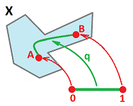
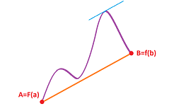
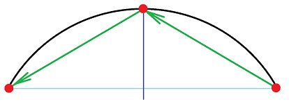
The picture suggests what happens to the entities we considered in Rolle's theorem: there is now a line that connects the end-points of the curve and this line is parallel to the tangent at some point!

Theorem (Mean Value Theorem). Suppose

• 1. $F$ is continuous on $[a,b]$,
• 2. $F$ is differentiable on $(a,b)$.

Then $$\frac{F(b) – F(a)}{b-a} = F'(c),$$ for some $c$ in $(a,b).$

Proof. The proof repeats the proof of the original Mean Value Theorem for numerical functions in Chapter 9. Let's rename $F$ in Rolle's Theorem as $H$ to use it later. Then its conditions take this form:

• 1. $H$ continuous on $[a,b]$,
• 2. $H$ is differentiable on $[a,b]$,
• 3. $H(a) = H(b)$.

Suppose $X=L(t)$ is a parametric curve represented by the straight line from $F(a)$ to $F(b)$ with $L(a)=F(a)$ and $L(b)=F(b)$. Then its derivative is simply its direction vector: $$L'(t)=\frac{F(b) – F(a)}{b-a}.$$ The key step is to define $h$ as the difference of these two parametric curves: $$H(x) = F(x) – L(x).$$ We now verify the conditions above. 1. $H$ is continuous on $[a,b]$ as the difference of the two continuous functions (SR). 2. $H$ is differentiable on $(a,b)$ as the difference of the two differentiable functions (SR): $$H'(x)=F'(x)-\frac{F(b) – F(a)}{b-a}.$$ 3. We also have: $$F(a) = L(a), \ F(b) = L(b)\ \Longrightarrow\ H(a) = 0,\ H(b) = 0\ \Longrightarrow\ H(a) = H(b).$$ Thus, $H$ satisfies the conditions of Rolle's Theorem. Therefore, the conclusion is satisfied too: $$H'(c)=0$$ for some $c$ in $(a,b)$; i.e., $$F'(c)-\frac{F(b) – F(a)}{b-a}=0.$$ $\blacksquare$

Geometrically, $c$ is found by shifting the displacement vector until it touches the graph:

The derivative is defined as the limit of the difference quotient; now we also have a back link. Indeed, what if we take the partition of $[a,b]$ to trivial: $n=1,\ x_0=a,\ x_1=b$? The theorem simply states that the two are equal, provided we choose the right point where to sample the derivative. For an arbitrary partition, we carry out the construction for each interval of the partition, as follows.

Corollary. Suppose

• 1. $F$ is continuous on $[a,b]$,
• 2. $F$ is differentiable on $(a,b)$.

Then for any partition of the interval $[a,b]$, there are such secondary nodes $c_1,...,c_n$ that $$\frac{\Delta F}{\Delta x}(c_k)=F'(c_k), \ k=1,2,...,n.$$

In other words, the directions of the lines connecting the points of the path of $F$ at the nodes of the partition are equal to the values of the derivative at the secondary nodes between them:

The Mean Value Theorem will help us to derive facts about the function from the facts about its derivative. Before the Mean Value Theorem, we have only been able to find facts about the derivative from the facts about the parametric curve. This is a short list of familiar facts: $$\begin{array}{l|l|ll} \text{info about }F &&\text{ info about }F'\\ \hline F\text{ is constant }&\Longrightarrow &F' \text{ is zero}\\ &\overset{?}{\Longleftarrow}&\\ \hline F\text{ is linear}&\Longrightarrow &F' \text{ is constant}\\ &\overset{?}{\Longleftarrow}&\\ \hline F\text{ is quadratic}&\Longrightarrow &F' \text{ is linear}\\ &\overset{?}{\Longleftarrow}&\\ \hline \end{array}$$ Are these arrows reversible? If the derivative of the function is zero, does it mean that the function is constant?

Consider this simple statement about motion:

• “if my velocity is zero, I am standing still”.

If $X=F(t)$ represent the position, we can restate this mathematically. The theorem is identical to the one in Chapter 7, but the constant is a vector this time!

Theorem (Constant). (A) If a parametric curve defined at the nodes of a partition of interval $[a,b]$ has a zero difference quotient for all nodes in the partition, then this function is constant over the nodes of $[a,b]$; i.e., $$\frac{\Delta F}{\Delta t}(c) = 0 \ \Longrightarrow\ F=\text{ constant }.$$ (B) If a differentiable on open interval $I$ function has a zero derivative for all $t$ in $I$, then this function is constant on $I$; i.e., $$F'=0 \ \Longrightarrow\ F=\text{ constant }.$$

Proof. (A) $$\frac{\Delta F}{\Delta x}(c_i) = 0 \ \Longrightarrow\ F(t_{i})-F(t_{i-1})=0\ \Longrightarrow\ F(t_{i})=F(t_{i-1}).$$ (B) To prove that $f$ is constant, it suffices to show that $$F(a) = F(b),$$ for all $a,b$ in $I$. Assume $a < b$ and use the Mean Value Theorem with interval $(a,b)$ inside the interval $I$: $$\frac{F(b) – F(a)}{b-a} =F'(c),$$ for some $c$ $(a,b)$. This is $0$ by assumption. Therefore, we have for all pairs $a,b$ in $I$: $$\frac{F(b) - F(a)}{b-a} = 0\ \Longrightarrow\ F(b) – F(a) = 0\ \Longrightarrow\ F(a) = F(b).$$ $\blacksquare$

Exercise. What if $F'=0$ on a union of two intervals?

The problem then becomes one of recovering the function $F$ from it derivative $F'$, the process we have called anti-differentiation. In other words, we reconstruct the function from a “field of vectors” (i.e., a vector field):

Now, even if we can recover the function $F$ from it derivative $F'$, there many others with the same derivative, such as $G=F+C$ for any constant real number $C$. Are there others? No.

Theorem (Anti-differentiation). (A) If two parametric curve defined at the nodes of a partition of interval $[a,b]$ have the same difference quotient, they differ by a constant vector; i.e., $$\frac{\Delta F}{\Delta x}(c) = \frac{\Delta G}{\Delta x}(c) \ \Longrightarrow\ F(x) – G(x)=\text{ constant }.$$ (B) If two differentiable on open interval $I$ parametric curves have the same derivative, they differ by a constant vector; i.e., $$F'(x) = G'(x) \ \Longrightarrow\ F(x) – G(x)=\text{ constant }.$$

Proof. Define $$H(t) = F(t) – G(t).$$ Then, by SR, we have: $$H'(t) = \left( F(t)–G(t) \right)'=F'(t)–G'(t) =0,$$ for all $x$. Then $H$ is constant, by the Constant Theorem. $\blacksquare$

Geometrically, this means that shifting the graph of $F$ gives us the graph of $G$.

The theorem represents a less obvious fact about motion:

• “if two runners run with the same velocity, their relative location isn't changing”.

Sums and integrals

Let's visualize what it means to differentiate and integrate a parametric curve.

Suppose our parametric curve $X=F(t),\ a\le t\le b$, is defined at these points: $X_i=F (t_i)$, where $t_{i+1}=t_i+h,\ i=1,2,...,n$. Between these locations we draw the displacement vectors, $D_i=X_iX_{i+1}$. We then move them so that the starting points are all the same, at the origin. We have created the vectors of displacement. By tracing the ends of these vectors we acquire a sequence of “locations” in this new space. The result is the difference of $X=F(t)$.

We can also re-scale these vector all at once: $V_i=\frac{1}{h}D_i,\ i=1,2,...,n$, producing the vectors of average velocity. The result is the difference quotient of $X=F(t)$.

If the points came from a sampled parametric curve, the limit $h\to 0$ finishes the job: we have a new parametric curve, $Q=G(t)$, the derivative of $X=F(t)$.

Now in reverse.

Suppose a parametric curve $Q=G(t),\ a\le t\le b$, is defined at these points: $Q_i=G(t_i)$, where $t_{i+1}=t_i+h,\ i=1,2,...,n$. We represent these “locations” as vectors $D_i=OQ_i$ starting at the same point, the origin. We think of them as displacements. We arrange them head-to-tail starting at some location $X_0$ producing a sequence of locations: $X_{i+1}=X_i+D_i,\ i=1,2,...,n$. The result is the sum of $Q=G(t)$.

If we instead think of the original vectors as velocities, we re-scale these vectors all at once first: $D_i=L_ih$, producing the displacement vectors. We arrange them head-to-tail starting at some location $X_0$ producing a sequence of locations: $X_{i+1}=X_i+D_i,\ i=1,2,...,n$. The result is the Riemann sum of $Q=G(t)$.

If the points came from a sampled parametric curve, the limit $h\to 0$ finishes the job: we have a new parametric curve $X=F(t)$, the integral of $Q=G(t)$.

The following is the general setup for sums and Riemann sums.

Suppose we have a parametric curve $X = F(t)$, maybe continuous maybe not, defined on $[a,b],\ a < b$. We start with an augmented partition of the interval. Given an integer $n \geq 1$, we have a partition of $[a,b]$ into $n$ intervals of possibly different lengths: $$ [t_{0},t_{1}],\ [t_{1},t_{2}],\ ... ,\ [t_{n-1},t_{n}],$$ with $t_0=a,\ t_n=b$. The intervals can be possibly reversed!

The points, $$t_{0},\ t_{1},\ t_{2},\ ... ,\ t_{n-1},\ t_{n},$$ will be called the nodes of the partition. The lengths of the intervals are: $$\Delta t_i = t_i-t_{i-1},\ i=1,2,...,n.$$ We are also given the secondary nodes: $$ c_{1} \text{ in } [t_{0},t_{1}], \ c_{2} \text{ in } [t_{1},t_{2}],\ ... ,\ c_{n} \text{ in } [t_{n-1},t_{n}].$$ The secondary nodes can be chosen to be the left- or the right-end points of the intervals, or the mid-points, etc.

Definition. The sum of a parametric curve $Q=G(t)$ over an augmented partition of an interval $[a,b]$ is defined to be $$\sum_a^b G =G(c_{1}) + G(c_{2}) + ... + G(c_{n})=\sum_{i=1}^{n} G(c_{i}). $$

Definition. The Riemann sum of a parametric curve $Q=F(t)$ over an augmented partition of an interval $[a,b]$ is defined to be $$\sum_a^b F \, \Delta t =F(c_{1})\, \Delta t_1 + F(c_{2})\, \Delta t_2 + ... + F(c_{n})\, \Delta t_n=\sum_{i=1}^{n} F(c_{i})\, \Delta t_i. $$

The sum may be illustrated as below for the $1$-dimensional case:

In higher dimensions, the Riemann sum is a combination of the areas of the rectangles with bases $[t_i,t_{i+1}]$ and heights produced by the components of $F(c_i)$.

Theorem (Constant Function Rule). Suppose $Q=F(t)$ is constant on $[a,b]$; i.e., $F(t) = C$ for all $t$ in $[a,b]$ and some vector $C$. Then $$\sum_{a}^{b} F\, \Delta t = C ( b-a ). $$

Now, in order improve these approximations, we refine the partition and keep refining; i.e., we have simultaneously: $$n \to \infty \text{ and } \Delta t_i \to 0.$$

Specifically, we define the mesh of a partition $P$ as: $$|P|=\max_i \, \Delta t_i.$$ It is a measure of “refinement” of $P$.

Definition. The Riemann integral of a parametric curve $F$ over interval $[a,b]$ is defined to be the limit of a sequence of its Riemann sums over a sequence partitions $P_k$ with their mesh approaching $0$ as $k\to \infty$. When all these limits exist and are all equal to each other, $F$ is called integrable over $[a,b]$ and the limit is denoted by: $$ \int_{a}^{b} F\, dt =\lim_{k \to \infty} \sum_a^b F_k \, \Delta t,$$ where $F_k$ is $F$ sampled at the secondary nodes of $P_k$. It is also called the definite integral of $F$. The interval $[a,b]$ is the domain of integration.

Theorem (Constant Integral Rule). Suppose $F$ is constant on $[a,b]$, i.e., $F(t) = C$ for all $t$ in $[a,b]$ and some vector $C$. Then $F$ is integrable on $[a,b]$ and $$\int_{a}^{b} F\, dt = C (b-a).$$

The following result proves that our definition makes sense for a large class of parametric curves.

Theorem. All continuous parametric curves on $[a,b]$ are integrable on $[a,b]$.

Theorem. The Riemann integral of a parametric curve $F$ over interval $[b,a]$ is equal to the negative of the integral over $[a,b]$: $$\int_{b}^{a} F\, dt =-\int_{a}^{b} F\, dt .$$

Exercise. Prove the theorem.

The Fundamental Theorem of Calculus

What is the opposite of subtraction? Addition. Then the opposite of the difference is the sum: $$\left. \begin{array} {rllll} \text{difference, } \Delta F:& \text{ vector subtraction } \\ & && \\ \text{sum, } \sum_a^t F :& \text{ vector addition } \end{array} \right\}\text{opposite!} $$ The two operations cancel each other!

Theorem (Fundamental Theorem of Discrete Calculus of degree $1$). Suppose $F$ is a parametric curve defined at the nodes of a partition of an interval $[a,b]$ and suppose $a$ is a node of the partition. Then, for each node $t$, we have $$\sum_a^t (\Delta F) =F(t)-F(a).$$

The components of the differences and the sum are the differences and sum of component functions as defined in Chapter 14. The relation we observed then now appears separately for each component:

We take this idea further and examine the fundamental relation between the Riemann sums and the difference quotients. It is only slightly more complicated.

In our vector-valued setting, let's take another look at the computations of motion.

First, this is how we use the velocity function to acquire the displacement. Then we discover that each of the values of the latter is a Riemann sum of the former!

Indeed, suppose we have a parametric curve $G$ defined at the secondary nodes of a partition of an interval $[a,b]$, i.e., a $1$-form with values in ${\bf R}^n$. Its Riemann sum defines a new parametric curve $\Gamma$ on the nodes, i.e., a $0$-form. It can be computed directly: $$\Gamma (t_k)=\sum_a^{t_k} G \, \Delta t,$$ or recursively: $$\Gamma (t_{k+1})=\Gamma (t_k)+G(c_k) \, \Delta t_k.$$

Second, this is how we use the parametric curve of location to acquire the velocity. Then we discover that each of the values of the latter is a difference quotient of the former!

Indeed, suppose we have a parametric curve $\Phi$ at the primary nodes of a partition of an interval $[a,b]$, i.e., a $0$-form with values in ${\bf R}^n$. Its difference quotient is computed over each segment of the partition $[t_{k-1},t_{k}],\ k=1,2,...,n$, and assigned to the corresponding secondary node $c_k$. This defines a new parametric curve $F$ on the secondary nodes, i.e., a $1$-form. It is computed by the familiar formula: $$F(c_{k})=\frac{\Phi (t_{k})-\Phi (t_{k-1})}{\Delta t_k}.$$

We realize that the difference quotients of the Riemann sums give us the original parametric curve; we just substitute the recursive formula for the latter into the last formula for the former: $\Phi =\Gamma $. Then we have: $$\begin{array}{lll} F(c_{k})&=\frac{\Gamma (t_{k})-\Gamma (t_{k-1})}{\Delta t_k}\\ &=\frac{G(c_k)\Delta t_k}{\Delta t_k}\\ &=G(c_k). \end{array}$$

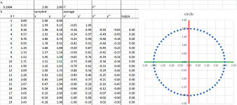
The result is seen in the spreadsheet below:

Now, vice versa, the Riemann sums of the difference quotients give us the original -- up to a constant vector -- parametric curve; we just substitute the last formula for the former into the recursive formula for the latter: $G(c_k)=F(c_k)$. If we assume that $\Gamma (t_k)= \Phi (t_k)+C$ for all $k$, the we conclude: $$\begin{array}{lll} \Gamma (t_{k})&=\Gamma (t_{k-1})+F(c_k)\Delta t_k\\ &=\Gamma (t_{k-1})+\frac{\Phi (t_{k})-\Phi (t_{k-1})}{\Delta t_k}\Delta t_k\\ &=\Gamma (t_{k-1})+ \Phi (t_{k})-F(t_{k-1})\\ &=\Phi (t_{k})+C. \end{array}$$

Let's summarize what we have proven -- for discretely defined parametric curves, i.e., a $0$- and $1$-forms with values in ${\bf R}^n$.

Definition. Suppose $\Phi$ is defined at the primary nodes $t_k,\ k=0,1,2,...,n$, of the partition. Then the difference quotient $F$ of $\Phi$ is defined at the secondary nodes of the partition by: $$F(c_{k})=\frac{\Phi (t_{k})-\Phi (t_{k-1})}{\Delta t_k};$$ it is denoted by $$F=\frac{\Delta \Phi}{\Delta t}.$$

Definition. Suppose $G$ is defined at the secondary nodes $c_k,\ k=1,2,...,n$, of the partition. Then the Riemann sum of $G$ is defined recursively at the primary nodes of the partition by: $$\Gamma (t_{k})=\Gamma (t_{k-1})+G(c_k)\Delta t_k;$$ it is denoted by: $$\Gamma =\sum_a^t G\, \Delta t.$$

Theorem (Fundamental Theorem of Discrete Calculus). (1) The difference quotient of the Riemann sum of $G$ is $G$: $$\frac{\Delta \left(\sum_a^t G \, \Delta t\right) }{\Delta t}=G.$$ (2) The Riemann sum of the difference quotient of $\Phi$ is $\Phi+C$, where $C$ is a constant: $$\sum_a^t\left( \frac{\Delta \Phi }{\Delta t} \right) \, \Delta t = \Phi (t)+C.$$

The two operations cancel each other! The result shouldn't be surprising considering the operations involved: $$\left. \begin{array} {rllll} \text{difference quotient, } \frac{\Delta F}{\Delta t}:& \text{ vector subtraction } &\to & \text{ scalar division } \\ & && \\ \text{Riemann sum, } \sum_a^t F \, \Delta t :& \text{ vector addition } &\gets & \text{ scalar multiplication } \end{array} \right\}\text{opposite!} $$

Now the continuous case. We just take the above relations and let $\Delta t$ approach $0$. We “zoom out” on the graph:

Definition. A parametric curve $X=F(t)$ is called an antiderivative of a parametric curve $Q=G(t)$ if $F'=G$. It is denoted by: $$G=\int F\, dt.$$

We use “an” because there are many antiderivatives for each parametric curve.

Theorem (Fundamental Theorem of Calculus). (1) Given a continuous parametric curve $Q=F(t)$ on $[a,b]$, the function defined by $$\Phi(x) = \int_{a}^{x} F \, dt $$ is an antiderivative of $F$ on $(a,b)$. (2) For a continuous parametric curve $Q=F(t)$ on $[a,b]$ and any of its antiderivatives $\Phi$, we have $$\int_{a}^{b} F \, dt =\Phi(b)-\Phi(a).$$

According to the Fundamental Theorem, the operations of differentiation and integration cancel each other: $$ \newcommand{\ra}[1]{\!\!\!\!\!\xrightarrow{\quad#1\quad}\!\!\!\!\!} \newcommand{\da}[1]{\left\downarrow{\scriptstyle#1}\vphantom{\displaystyle\int_0^1}\right.} % \begin{array}{ccccccccccccccc} F & \mapsto & \begin{array}{|c|}\hline\quad \int (\quad )\,dt \quad \\ \hline\end{array} & \mapsto & \Phi & \mapsto &\begin{array}{|c|}\hline\quad \frac{d}{dt}(\quad ) \quad \\ \hline\end{array} & \mapsto & F.\\ \Phi & \mapsto & \begin{array}{|c|}\hline\quad \frac{d}{dt}(\quad ) \quad \\ \hline\end{array} & \mapsto & F & \mapsto &\begin{array}{|c|}\hline\quad \int (\quad )\,dt\quad \\ \hline\end{array} & \mapsto & \Phi+C. \end{array}$$

Corollary. If $G$ is an antiderivative of $F$ then so is $G+C$, where $C$ is any constant vector.

Thus, of $X=F(t)$ and $X=G(t)$ are two antiderivatives of the same parametric curve, then not only their paths are the same, shifted by a fixed vector, but also the two locations $F(t)$ and $G(t)$ at the exact moment of time are also separated by that vector.

Algebraic properties of sums and integrals

Just as in dimension $1$ (Chapter 1), algebraic operations on functions produce algebraic operations on their sums. The properties for integrals follow from the corresponding properties of the sums and the rules of limits.

If we proceed to the adjacent interval, we can just continue to add terms of the sum (one component shown):

Theorem (Additivity Rule). (A) Suppose $F$ is a vector-valued function (parametric curve) defined at the nodes of a partition. Then, for any nodes $a,b,c$, we have: $$\sum_a^b F +\sum_b^c F = \sum_a^c F ,$$ and $$\sum_a^b F\, \Delta t +\sum_b^c F\, \Delta t = \sum_a^c F \, \Delta t,$$ over partitions of $[a,b]$, $[b,c]$, and $[a,c]$ respectively. (B) Suppose a vector-valued function (parametric curve) $F$ is integrable over $[a,b]$ and over $[b,c]$. Then $F$ is integrable $[a,c]$ and we have: $$\int_a^b F\, dt +\int_b^c F\, dt = \int_a^c F\, dt.$$

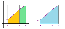
The area interpretation of additivity of integrals is the same:

With the motion interpretation, we have: $$\begin{array}{lll} &\text{displacement during the 1st hour }\\ +&\text{displacement during the 2nd hour }\\ =&\text{displacement the two hours}. \end{array}$$

Theorem (Estimate Rule). (A) Suppose $F$ is a vector-valued function (parametric curve) defined at the nodes of a partition. Then, for any nodes $a,b$ with $a<b$, if $$||F(x)||\leq M,$$ for all $t$ with $a\le t \le b$, then $$\left\Vert\sum_{a}^{b} F\, \Delta t \right\Vert \leq M(b-a).$$ (B) Suppose $F$ is an integrable vector-valued function (parametric curve) over $[a,b]$. Then, if $a<b$ and $$||F(x)||\leq M,$$ for all $t$ with $a\le t \le b$, we have $$\left\Vert \int_{a}^{b} F\, dt \right\Vert \leq M(b-a).$$

Note that the statement of the theorem still holds even if $F$ is integrable over $[b,a]$ with $b<a$, etc. This implies the following important result.

Theorem. If a vector-valued function (parametric curve) $F$ is integrable over $[a,b]$ then it is also integrable over any $[a',b']$ with $a\le a' < b' \le b$.

The following is another important corollary.

Theorem. All piece-wise continuous parametric curves are integrable.

These are the algebraic properties.

Theorem (Constant Multiple Rule). (A) Suppose $F$ is a vector-valued function (parametric curve) defined at the nodes of a partition. Then, for any nodes $a,b$ and any real $c$, we have: $$ \sum_{a}^{b} (c\cdot F) = c \cdot \sum_{a}^{b} F,$$ and $$ \sum_{a}^{b} (c\cdot F) \, \Delta t = c \cdot \sum_{a}^{b} F\, \Delta t.$$ (B) Suppose a vector-valued function (parametric curve) $F$ is integrable over $[a,b]$. Then so is $c\cdot f$ for any real $c$ and we have: $$ \int_{a}^{b} (c\cdot F)\, dt = c \cdot \int_{a}^{b} F\, dt.$$

Theorem (Sum Rule). (A) Suppose $F$ and $G$ are vector-valued functions (parametric curves) defined at the nodes of a partition. Then, for any nodes $a,b$, we have: $$\sum_{a}^{b} \left( F + G \right) = \sum_{a}^{b} F + \sum_{a}^{b} G, $$ and $$\sum_{a}^{b} \left( F + G \right) \, \Delta t = \sum_{a}^{b} F\, \Delta t + \sum_{a}^{b} G\, \Delta t. $$ (B) Suppose vector-valued functions (parametric curves) $F$ and $G$ are integrable over $[a,b]$. Then so is $F+G$ and we have: $$\int_{a}^{b} \left( F + G \right)\, dt = \int_{a}^{b} F\, dt + \int_{a}^{b} G\, dt. $$

The rate of change of the rate of change: the second difference quotient and the second derivative

While the original parametric curve was defined at the nodes of a partition, its difference and the difference quotient are defined at the secondary nodes. Following the ideas from Chapter 8, we treat the latter as functions that also have their own difference and difference quotient. What is the partition then? We saw earlier in the chapter how this idea is implemented in order to derive the acceleration from the velocity.

First, also following Chapter 8, we notice that the difference of the difference is simply the difference that skips a node. That's why the second difference doesn't provide us -- in this $1$-dimensional setting -- with any meaningful information. We will limit our attention to the difference quotients.

We need three values of the function $F$ at the nodes. We then compute the difference quotients along the two intervals and place the results within the corresponding edge. Finally, the same operation is carried out for these two values: $$\begin{array}{ccc} -&F(t_1)&---&F(t_2)&---&F(t_3)&-&\\ -&-\bullet-&\frac{\Delta F}{\Delta t_2}&-\bullet-&\frac{\Delta F}{\Delta t_3}&-\bullet-&-\\ -&-\bullet-&---&\frac{\frac{\Delta F}{\Delta t_3} -\frac{\Delta F}{\Delta t_2}}{c_3-c_2}&---&-\bullet-&-&\\ &t_1&c_2&t_2&c_3&t_3&\\ \end{array}$$ This is all vector algebra!

The function defined above represents the directions of the lines connecting the values of $F$ at consecutive nodes of the partition. In particular, when the location is represented by a function known only at the nodes of the partition, the (average) velocity is then found in this manner. It is now especially important that we have utilized the secondary nodes as the inputs of the new function. Indeed, we can now carry out a similar construction with this function and find the (average) acceleration!

We have now a new augmented partition, of what? The interval is $$[p,q],\ \text{ with } p=c_0 \text{ and } q=c_n.$$ We partition it into $n-1$ intervals with the help of the nodes that used to be the secondary nodes in the last partition: $$p=c_{1},\ c_{2},\ c_{3},\ ... ,\ c_{n-1},\ c_{n}=b.$$ When $c_k=c_{k+1}$, we exclude this “interval” from the new partition. Now, what are the secondary nodes? The primary nodes of the last partition of course! Indeed, we have: $$ t_{1} \text{ in } [c_{1},c_{2}], \ t_{2} \text{ in } [c_{2},c_{3}],\ ... ,\ t_{n-1} \text{ in } [c_{n-1},c_{n}].$$

We apply the same construction to this partition to the function $G=\frac{\Delta F}{\Delta t}$. The difference quotient function of $F$ is defined at the secondary nodes of the new partition (the primary nodes of the old partition) by the same formula: $$\frac{\Delta G}{\Delta t}(t_{k})=\frac{G(c_{k+1})-G(c_k)}{c_{k+1}-c_k}.$$

Definition. The second difference quotient of $X=F(t)$ is defined at the primary nodes of the partition by: $$\frac{\Delta^2 F}{\Delta t^2}(t_{k})=\frac{\frac{\Delta F}{\Delta t}(c_{k+1})-\frac{\Delta F}{\Delta t}(c_k)}{c_{k+1}-c_k},\ k=1,2,...,n-1.$$

It is then a vector-valued $0$-form.

Example. Let's find the second difference quotient of the standard parametrization of the circle, $$X(t)=<\cos t,\ \sin t>.$$ It was considered previously in this chapter: $$\frac{\Delta X}{\Delta t}(c)=\frac{ \sin (h/2)}{h/2}<-\sin c,\ \cos c>.$$ Here we have a mid-point partition for the interval, say, $[-\pi/2,\pi/2]$, in the $t$-axis:

• the nodes are $x=a,a+h,...$ and
• the secondary nodes are $c=a+h/2,...$.

Over the same mid-point partition, we have the second difference quotient: $$\frac{\Delta^2 X}{\Delta t^2}(a)=-\left(\frac{ \sin (h/2)}{h/2}\right)^2<\cos a,\ \sin a>.$$ This vector points toward the center of the circle! $\square$

The construction of the difference quotient is repeatedly used for approximations and simulations which is followed, when necessary, by taking its limit. The result is the derivative and the second derivative.

The derivative of a differentiable parametric curve is also a parametric curve and can also be differentiated.

The notation is identical to that for numerical functions: $$\begin{array}{|l|l|l|l|} \hline \text{function } & F & F^{(0)}&\\ \text{first derivative } & F' & F^{(1)}&\frac{dF}{dt}\\ \text{second derivative } & F' '=(F')' & F^{(2)}=\left(F^{(1)}\right)'&\frac{d^2F}{dt^2}=\frac{d}{dt}\left( \frac{dF}{dt} \right)\\ \text{third derivative } & F' ' '=(F' ')'& F^{(3)}=\left(F^{(2)}\right)'&\frac{d^3F}{dt^3}=\frac{d}{dt}\left( \frac{d^2F}{dt^2} \right)\\ ...&&...&...\\ n\text{th derivative } & & F^{(n)}=\left(F^{(n-1)}\right)'&\frac{d^nF}{dt^n}=\frac{d}{dt}\left( \frac{d^{n-1}F}{dt^{n-1}} \right)\\ ...&&...&...\\ \hline \end{array}$$ Thus, a given differentiable function may produce a sequence of parametric curves: $$ \newcommand{\ra}[1]{\!\!\!\!\!\xrightarrow{\quad#1\quad}\!\!\!\!\!} \newcommand{\da}[1]{\left\downarrow{\scriptstyle#1}\vphantom{\displaystyle\int_0^1}\right.} % \begin{array}{ccccccccccccccccc} F & \mapsto & \begin{array}{|c|}\hline\quad \tfrac{d}{dt} \quad \\ \hline\end{array} & \mapsto & F' & \mapsto & \begin{array}{|c|}\hline\quad \tfrac{d}{dt} \quad \\ \hline\end{array} & \mapsto & F' '& \mapsto & ...& \mapsto & F^{(n)}& \mapsto &... \end{array}$$ provided the outcome of each step is differentiable as well. In the abbreviated form the sequence is: $$\newcommand{\ra}[1]{\!\!\!\!\!\xrightarrow{\quad#1\quad}\!\!\!\!\!} \newcommand{\la}[1]{\!\!\!\!\!\xleftarrow{\quad#1\quad}\!\!\!\!\!} \newcommand{\da}[1]{\left\downarrow{\scriptstyle#1}\vphantom{\displaystyle\int_0^1}\right.} \newcommand{\ua}[1]{\left\uparrow{\scriptstyle#1}\vphantom{\displaystyle\int_0^1}\right.}\begin{array}{cccccccccccc} F &\ra{\frac{d}{dt}} &F' &\ra{\frac{d}{dt}} & F' ' &\ra{\frac{d}{dt}} &...&\ra{\frac{d}{dt}} & F^{(n)} &\ra{\frac{d}{dt}} & ... \end{array}$$

Warning: We will see in Chapter 18 that the function and its derivative are two animals of very different breeds in higher dimensions.

Definition. A parametric curve $F$ is called twice, thrice, ..., $n$ times differentiable when the corresponding derivatives, $$F',F' ',F' ' ',..., F^{(n)},$$ exist. When the derivatives exist for all $n$, we call the function smooth.

Example. Examples of functions that are differentiable but not twice differentiable come from Chapter 7: $$f(x)=\begin{cases} -x^2&\text{ if } x<0;\\ x^2&\text{ if } x\ge 0. \end{cases}$$

$\square$

Below we visualize the relation between these classes of functions. It is the same for numerical functions:

What is the geometric meaning of these higher derivatives?

The first derivative represents the direction and the magnitude of change of the vector-valued function. Then the second derivative represents the rate of change of these directions and these magnitudes. Notice how changing slopes are seen as rotating tangents:

It other words, this is acceleration.

Reversing differentiation: antiderivatives

Now in the vector algebra environment, we come back to the same question as in Chapter 7: when we know the velocity at every moment of time, how do we find the location? How do we “reverse” the effect of differentiation on a function?

For a parametric curve $X=G(t)$ defined at the secondary nodes, $c_k$, of a partition, the answer remains the same; we have an almost identical recursive formula for the parametric curve $X=F(t)$ defined at the nodes, $t_k$, of the partition: $$F(t_{k+1})= F(t_k+\Delta t_k)=F(t_k)+G(c_k)\Delta t_k.$$ Then, $$\frac{\Delta F}{\Delta t_k}=G(c_k);$$ i.e., the difference quotient of $F$ is $G$.

What about the derivative? With the complexity added by the limit, there is no formula, even recursive. First, let's review how the Sum Rule, the Constant Multiple Rule, and the Chain Rule are represented as diagrams: $$\newcommand{\ra}[1]{\!\!\!\!\!\xrightarrow{\quad#1\quad}\!\!\!\!\!} \newcommand{\la}[1]{\!\!\!\!\!\xleftarrow{\quad#1\quad}\!\!\!\!\!} \newcommand{\da}[1]{\left\downarrow{\scriptstyle#1}\vphantom{\displaystyle\int_0^1}\right.} \newcommand{\ua}[1]{\left\uparrow{\scriptstyle#1}\vphantom{\displaystyle\int_0^1}\right.} \begin{array}{ccc} F,G&\ra{\frac{d}{dt}}&F',G'\\ \ \da{+}&SR &\ \da{+}\\ F+G & \ra{\frac{d}{dt}}&(F+G)'=F'+G' \end{array}\qquad \begin{array}{ccc} F&\ra{\frac{d}{dt}}&F'\\ \ \da{\cdot c}& CMR &\ \da{\cdot c}\\ cF & \ra{\frac{d}{dt}}&(cF)'=cF' \end{array}\qquad \begin{array}{ccc} F,G&\ra{\frac{d}{dt}}&F',G'\\ \ \da{\circ}& CR &\ \da{\circ }\\ F\circ G & \ra{\frac{d}{dt}}&(F\circ G)'=F'\circ G' \end{array} $$ In the first diagram, we start with a pair of functions at the top left and then we proceed in two ways:

• right: differentiate, then go down: add the results; or
• down: add them, then go right: differentiate the result.

The result is the same! (Neither the Product Rule nor the Quotient Rule has such an interpretation.)

Now, anti-differentiation is meant to “reverse” the effect of differentiation on a function just as before. It is similar to the inverse of a function.

The importance of this “inverse” problem stems from the need to find location from velocity or velocity from acceleration. For example, this is what we derive from our experience with differentiation of parametric curves:

• the acceleration is constant, $A$ $\Longrightarrow$
• the velocity is a linear function, $V(t)=At+B$ $\Longrightarrow$
• the location is a quadratic function, $X(t)=At^2/2+Bt+C$.

Here $B$ and $C$ are the initial velocity and the initial position respectively.

We illustrate the idea with a diagram: $$ \newcommand{\ra}[1]{\!\!\!\!\!\xrightarrow{\quad#1\quad}\!\!\!\!\!} \newcommand{\da}[1]{\left\downarrow{\scriptstyle#1}\vphantom{\displaystyle\int_0^1}\right.} % \begin{array}{ccccccccccccccc} <t^2,\ t^3> & \mapsto & \begin{array}{|c|}\hline\quad \tfrac{d}{dt} \quad \\ \hline\end{array} & \mapsto & <2t,\ 3t^2>; \\ <2t,\ 3t^2> & \mapsto & \begin{array}{|c|}\hline\quad \left( \tfrac{d}{dt}\right)^{-1} \quad \\ \hline\end{array} & \mapsto & <t^2+C,\ t^3+K> \end{array}$$ As a function, $\tfrac{d}{dt}$ isn't one-to-one!

We will need the rules of anti-differentiation.

First, consider SR: $(F + G)' = F' + G'$. Let's read from right to left.

Theorem (Sum Rule). If

• $F$ is an antiderivative of $P$ and
• $G$ is an antiderivative of $Q$,

then

• $F+G$ is an antiderivative of $P+Q$.

Proof. We apply SR: $$\left( F(x)+G(x) \right)'= F'(x)+G'(x)=P(x)+Q(x).$$ $\blacksquare$

Similarly, we acquire the following.

Theorem (Constant Multiple Rule). If

• $F$ is and antiderivative of $P$ and
• $c$ is a constant,

then

• $cF$ is an antiderivative of $cP$.

Proof. We apply CMR: $$\left( cF(x) \right)'= cF'(x)=cP(x).$$ $\blacksquare$

Example. Find an antiderivative of ... $\square$

Theorem (Linear Chain Rule). If

• $F$ is and antiderivative of $P$ and
• $a\ne 0,\ b$ are constants,

then

• $\tfrac{1}{a}F(ax+b)$ is an antiderivative of $P(ax+b)$.

Proof. We apply CMR and CR: $$\left( \tfrac{1}{a}F(ax+b) \right)'=\tfrac{1}{a} \left( F(ax+b) \right)'=\tfrac{1}{a} a F'(ax+b)=F'(ax+b)=P(ax+b).$$ $\blacksquare$

These diagrams illustrate how differentiation and anti-differentiation undo each other: $$ \newcommand{\ra}[1]{\!\!\!\!\!\xrightarrow{\quad#1\quad}\!\!\!\!\!} \newcommand{\da}[1]{\left\downarrow{\scriptstyle#1}\vphantom{\displaystyle\int_0^1}\right.} % \begin{array}{ccccccccccccccc} F & \mapsto & \begin{array}{|c|}\hline\quad \left( \tfrac{d}{dt}\right)^{-1} \quad \\ \hline\end{array} & \mapsto & F & \mapsto &\begin{array}{|c|}\hline\quad \tfrac{d}{dt} \quad \\ \hline\end{array} & \mapsto & F,\\ F & \mapsto & \begin{array}{|c|}\hline\quad \tfrac{d}{dt} \quad \\ \hline\end{array} & \mapsto & F & \mapsto &\begin{array}{|c|}\hline\quad \left( \tfrac{d}{dt}\right)^{-1} \quad \\ \hline\end{array} & \mapsto & F+C. \end{array}$$ Just as with the numerical functions, there is a constant of integration but this time it is a vector.

We restate the rules.

Sum Rule: $$\int (F+G)dt=\int F\, dt+\int G\, dt.$$

Constant Multiple Rule: $$\int (cF)dt=c\int F\, dt.$$

Linear Chain Rule: $$\int F(mt+b)dt=\tfrac{1}{m}\int F(u)\, du\Big|_{u=mt+b}.$$

At least, we have these two diagrams to illustrate the interaction of antiderivatives with algebra: $$\newcommand{\ra}[1]{\!\!\!\!\!\xrightarrow{\quad#1\quad}\!\!\!\!\!} \newcommand{\la}[1]{\!\!\!\!\!\xleftarrow{\quad#1\quad}\!\!\!\!\!} \newcommand{\da}[1]{\left\downarrow{\scriptstyle#1}\vphantom{\displaystyle\int_0^1}\right.} \newcommand{\ua}[1]{\left\uparrow{\scriptstyle#1}\vphantom{\displaystyle\int_0^1}\right.} \begin{array}{ccc} P,Q&\la{\int}&F',G'\\ \ \da{+}& &\ \da{+}\\ P+Q & \la{\int}&F'+G' \end{array}\qquad \begin{array}{ccc} P&\la{\int}&F'\\ \ \da{\cdot c}& &\ \da{\cdot c}\\ cP & \la{\int}&cF' \end{array}$$ We start with a pair of functions at top right and proceed in two ways:

• left: anti-differentiate them, then go down: add the results; or
• down: add them, then go left: anti-differentiate the results.

The result is the same!

Theorem (Component-wise integration). The components of an antiderivative are the antiderivatives of the components: $$\int <f_1(t),...,f_n(t)>\, dt= <\int f_1(t)\, dt,...,\int f_n(t)\, dt>.$$

Example. Let's integrate: $$\begin{array}{llll} \int <\cos t,\ \sin t>\, dt&= <\int\cos t\, dt,\ \int\sin t\, dt>\\ &=<\sin t+C,\ \cos t+K>\\ &=<\sin t,\ \cos t>+<C,K>. \end{array}$$ Here $C$ and $K$ are just arbitrary constants which makes $<C,K>$ just an arbitrary vector. $\square$

The speed

Driving at a constant speed allows one to appreciate the scenery... and to study the shape of the road!

We already know that if we are moving in such a way that the distance to the origin remains the same, then our velocity is always perpendicular to the vector of location.

For the discrete case: $$||F(t)||=r\ \Longrightarrow\ \frac{\Delta F}{\Delta t}(t) \cdot\bigg( F(t+\Delta t)+F(t)\bigg)=0.$$ This means that the difference quotient $\frac{\Delta F}{\Delta t}$ is perpendicular to the average of the two consecutive locations. For the continuous case: $$||F(t)||=r\ \Longrightarrow\ F'\cdot F=0.$$

What about the relation between the velocity and the acceleration?

Suppose the difference quotient has a constant magnitude. Then we make an important geometric observation: the median of an isosceles is also its height.

Therefore, the velocity, in a sense, is perpendicular to the acceleration.

Now, the derivatives. We see the following as the velocity and the acceleration of the motion along the circle: $$F'(t)=<-\sin t,\ \cos t>\text{ and } F' '(t)=<-\cos t,\ -\sin t> .$$ Therefore: $$F'(t)\perp F' '(t).$$

For the general case, we suppose that our motion given by $X=F(t)$ is conducted in such a way that the speed remains the same: $$||F'(t)||=s.$$ Then, $$\frac{d}{dt}||F'||^2=0\ \Longrightarrow\ \frac{d}{dt}\big(F'\cdot F'\big)=0\ \Longrightarrow\ F' '\cdot F'+F'\cdot F' '=0\ \Longrightarrow\ F' '\cdot F'=0.$$

So, our acceleration is always perpendicular to the velocity. The advantage of this reformulation is that is applicable to all dimensions!

Warning: Just because the magnitude of the velocity is constant doesn't mean that the magnitude of the acceleration is zero (or even constant). The latter will depend on the sharpness of the turn, i.e., the curvature of the curve.

If we compare the result to the example we started with, we realize that it is as if -- at every moment of time -- we are moving along a circle at a constant speed and the acceleration points to the center of this circle.. but the circles are constantly changing!

We now realize that not only the relation between two pairs of parametric curves is the same (a function and its derivative) but also that the two computations are exactly the same!

Theorem. (A) For any parametric curve $U=G(t)$ defined at the nodes of a partition, we have: $$||G||=r>0\ \Longrightarrow\ \frac{\Delta G}{\Delta t}(c)\perp \frac{G(t)+G(t+\Delta t)}{2},$$ where $c$ is the corresponding secondary node, provided $\Delta G(c)\ne 0$. (B) For any differentiable parametric curve $U=G(t)$, we have: $$||G||=r>0\ \Longrightarrow\ \frac{dG}{dt}\perp G,$$ provided $\frac{dG}{dt}\ne 0$.

Driving at a constant speed, we never feel pressed into our seat or the seat belt but only feel the side-to-side swing. A constant speed parametrization takes the magnitude of the velocity -- how fast we progress forward -- out of consideration and allows us to concentrate on the curvature -- how fast the direction is changing. As all regular curves have such parametrizations, they will be a major tool of our study of their shapes!

Curves vs. parametric curves

We now transition from studying driving to studying roads. In mathematical terms, we transition from parametric curves to curves. But what is a curve?

Definition. A curve $C$ in ${\bf R}^n$ is the path of a continuous parametric curve, called its parametrization.

Then a curve is the combination of all of its parametrizations and we will need to answer the question: what do all these parametrizations have in common?

Suppose we have two parametrizations $X=G(s)$ and $X=F(t)$ of curve $C$. How are they related to each other?

A change of variables is a function used for substitution: $$t=g(s),$$ that turns one into the other: $$G(s)=F(g(s)).$$ This composition is seen in this commutative diagram: $$\newcommand{\ra}[1]{\!\!\!\!\!\xrightarrow{\quad#1\quad}\!\!\!\!\!} \newcommand{\ua}[1]{\left\uparrow{\scriptstyle#1}\vphantom{\displaystyle\int_0^1}\right.} % \begin{array}{cccccccccc} [a,b] & \ra{F} & {\bf R}^n \\ \ua{g} & \nearrow_G & \\ [c,d] & & \end{array}$$ Then, if $F$ is a parametrization of $C$, $G$ is called a re-parametrization.

We know that as long as the function $t=g(s)$ of the change of variables is one-to-one and onto, the new path will be the same as the old. It's as if a driver made a recording of his drive along the road and we just run it at a different (possible variable) speed. However, this is only possible when the driver didn't stop or turned around.

Definition. Suppose $X=F(t)$ is a parametric curve defined on $[a,b]$. If

• $F$ is differentiable on $(a,b)$,
• $F'$ is continuous on $(a,b)$, and
• $F'\ne 0$ on $(a,b),$

the curve is called regular. It is called a regular parametrization of the path.

Now, what if the two drivers drove in the opposite directions?

The curvature

We would like to devise a way to evaluate sharpness of turns of the road:

Since, depending on the car, we may need smaller or larger turning circles, we will know if this is possible.

If we progress incrementally, the curvature is simply the turn that we make at each step. At its simplest, the road is a city street. We then move from intersection to intersection.

These are the only options: $$\begin{array}{llc} \text{turn}&\text{rotation}&\text{}\\ \hline \text{no turn}&0 \text{ degrees}&0\\ \text{left turn}&90 \text{ degrees}&\pi/2\\ \text{right turn}&90 \text{ degrees}&\pi/2\\ \text{U-turn}&180 \text{ degrees}&\pi\\ \end{array}$$ How do we find the angle? We copy each vector, attach the copy to its end point, and compare to the next vector. Does this mean that the curvature a $90$-degree turn is $\pi/2$? No, because, as we know, the curvature scales down as the curve is scaled up, proportionally.

In order to measure the curvature in a scale independent manner, we use the angle of turn per distance covered, specifically, the distance between their centers of the two edges. For example, on the standard grid with edges of length $1$, this distance is $\frac{\sqrt{2}}{2}$ and, therefore, the curvature of a $90$-degree turn is $\frac{\pi}{\sqrt{2}}$. It is when the diagonal of the grid is $1$, we have the curvature of such a turn equal to $\pi/2$.

Example (square and circle). Let's confirm that this approach makes sense by considering a square and circle. We plot the unit circle, $$F(t)=<\cos t,\ \sin t>,$$ with $n$ points. For $n=4$, we have a square with a unit diagonal.

Here, we see the following columns. We compute the locations, then displacement for each two locations, then normalize them, then compute the angle between them (as the arccosine of their dot product), then finally divide by the half of the magnitude of the difference of the two displacements. The result is that the curvature is $\pi/2$.

Now, for $n=100$, we have something very close to a unit circle. Through the same computations, the curvature is $1$.

This means that we have to turn $\pi$ radians per $\pi$ units of lengths traveled. Changing the radius from $1$ to $2$ makes the curvature become $1/2$. $\square$

Now, suppose we have three distinct points $P_1,P_2,P_3$ in ${\bf R}^n$. What is the meaning of the curvature of this “curve”? It's not just its angle at $P_2$, i.e., $\widehat{P_1P_2P_3}$, but the angle the vectors $P_1P_2$ and $P_1P_2$ divided by the distance between their centers. We can choose to measure the turn not as an angle but rather the difference of the two vectors.

Suppose a sequence $C$ of distinct points in ${\bf R}^n$ is represented by a parametric curve $X_k=F(t_k)$ defined at the nodes of a partition. Let's try this formula for the curvature of a parametric curve: $$\varkappa(c_k)=\left| \frac{\big(F(t_k)-F(t_{k-1})\big) - \big( F(t_{k+1})-F(t_{k}) \big) }{(F(t_{k+1})-F(t_{k-1}))/2}\right|.$$

Example (circle). We apply the formulas to the standard parametrization: $$F(t)=<2\cos t,\ 2\sin t>.$$

The curvature is $1/2$ as expected. $\square$

We recognize some of these computations as difference quotients... Let's try this formula for the curvature of a parametric curve: $$\varkappa=\left| \frac{\Delta }{\Delta t}\left( \frac{\Delta T}{\Delta t} \right)\right|.$$ where $T$ is the normalized vector of the velocity.

Example (circle). The curve $X=F(t)$ is sampled in the two columns marked $x$ and $y$ and then use the difference quotient to get the average velocity $\frac{\Delta F}{\Delta t}$ in the columns marked $x'$ and $y'$. This time, we compute the speed $s$ as the magnitude of this vector and then normalize the velocity to get the unit tangent vector $T$: $$\texttt{=RC[-3]/RC8} \ .$$ It is plotted to confirm that the vectors are of length $1$:

We use the difference quotient again to get the average rate of change of $T$ and put it into the columns marked $T'x$ and $T'y$. It is also plotted. Finally, the magnitude of this vector is computed divided by the speed $s$; that's the curvature. It is constant at $1/2$ as expected. A parametrization with a non-constant speed produces the same result:

$\square$

Example (ellipse). We use the same spreadsheet for ellipses... We get the average speed of $T$ and plot it:

We recognize that at the start -- at $(1,0)$ -- we have a vertical tangent vector and then it turns counterclockwise. The magnitude of this vector is computed divided by the speed $s$; that's the curvature. It is also plotted:

We can see how it is low at first at the flatter end of the ellipse and then grows to a larger value as we reach the sharper end. It runs between $1/4$ and $2$. Two circles with radii $4$ and $1/2$ are seen to approximate the ellipse at its two ends:

$\square$

The arc-length parametrization

The main interest about these roads is their curvature: is the turn too sharp so that the motorists may have trouble to staying on the road at a particular speed? How can we find out? There is no other way to learn the shape of the road but to drive over it! We are back to drivers, but what kinds of drivers are best for our purposes?

Imagine yourself driving. At first the road is straight which is recognized by the fact that you see a tree ahead and continue to see it to remain straight ahead. Then, as you start to turn, the trees start to pass your field of vision from right to left:

The trees may pass faster or slower. When it is faster, does it mean that the curvature of the road is higher? Not necessarily! Maybe you are just driving faster... So, we don't want drivers who drive erratically: speed up and slow down, or stop, or even turn around. The perfect driver for the job drives at a constant speed!

Example (circle). The standard parametrization of the circle of radius $2$ is: $$F(t)=<2\cos t,\ 2\sin t>.$$ However, we cover the whole circle -- length $4\pi$ -- in $2\pi$ seconds. Let's slow down -- by a factor of $2$ -- and drive with speed $1$! This is how: $$G(t)=<2\cos (t/2),\ 2\sin (t/2)>.$$ Then in the formula for the curvature of a parametric curve discussed in the last section the normalization step disappears and the two difference quotients merge into the second difference quotient: $$\varkappa=\left\Vert \frac{\Delta^2 G}{\Delta t^2} \right\Vert.$$ For computations, we apply the difference quotient twice and then find the magnitude of the resulting vector:

The curvature is $1/2$ as expected. $\square$

At its simplest, the motion is described by the following two concepts: $$\begin{array}{|lll|l|l|} \hline \text{velocity} &= \frac{\text{displacement}}{\text{time}}&&\text{vectors}&\text{parametric curves}\\ \hline \text{speed} &= \frac{\text{distance}}{\text{time}}&= \frac{||\text{displacement}||}{\text{time}}&\text{numbers}&\text{numerical functions}\\ \hline \end{array}$$

The familiar way to look at the curvature is to measure how much the curve deviates from a straight line. But what line is that? There is no single line! At every location we will look at how much our motion takes us away from the current tangent line.

The curvature is then a measure of how fast the direction is changing. It is then the measure of how fast the tangent line is turning. Note that this is not the same as to say that the curvature is how fast the tangent vector, $F'$, is changing, which is $F' '$, as this would make the concept dependent on the speed, $||F'||$. Unless, of course, the speed is fixed at, say, $1$. In that case, we are measuring the speed of turning of a unit vector.

It is the same as the rate of change of this vector. Thus, for a “unit-speed” parametrization $X=G(s)$, i.e., $||G'||=1$, the curvature is the rate of change of the velocity vector $G'$, i.e., the acceleration.

Definition. Suppose a parametrization $X=G(s)$ of a curve $C$ satisfies $||G'||=1$, then the curvature of the curve is the numerical function that is the magnitude of the vector function of the second derivative: $$\varkappa(t)=||G' '(t)||.$$

Example (curvatures of circles). Let's compare two circles of radius $2$ and radius $1$. Now, over the same distance, $\pi$, and, therefore, over the same time, covered by a point moving at speed $1$ the rotation of the tangent is respectively $\pi/2$ and $\pi$:

The smaller circle has twice as large curvature! It seems that the curvature of a circle is the reciprocal of its radius... At the extreme, the large circle turns into a straight line with zero curvature! $\square$

Definition. A parametrization $X=G(s)$ is called an arc-length parametrization if $||G'(s)||=1$.

Example (circle). The standard parametrization of the circle of radius $R$ (a constant angular velocity), $$F(t)=<R\cos t,\ R \sin t>,$$ isn't arc-length unless $R=1$ because $$F'(t)=<-R\sin t,\ R \cos t> \ \Longrightarrow\ ||F'(t)||=\sqrt{(-R\sin t)^2+(R \cos t)^2}=R\sqrt{(\sin t)^2+(\cos t)^2}=R.$$ How can we make this into an arc-length parametrization? We have to be careful so that the modified curve is still the circle. The safest way to ensure that is to re-scale the time $t$. From the last example: we have to move slower if $R<1$ and faster if $R>1$. What should we replace $t$ with so that $R$ is cancelled under differentiation? Just put: $$t=s/R.$$ Then, indeed, we have $$G(s)=<R\cos (s/R),\ R \sin (s/R)> \ \Longrightarrow\ G'(s)=<-\sin (s/R),\ \cos (s/R)> \ \Longrightarrow\ ||G'(s)||=1,$$ by the Pythagorean Theorem. $\square$

Example (line). Let's consider this line: $$F(t)=<3,4>t\ \Longrightarrow\ F'(t)=<3,4>\ \Longrightarrow\ ||F'(t)||=\sqrt{3^2+4^2}=5.$$ How can we make this into an arc-length parametrization? We re-scale the time $t$ again to slow it down: $$t=s/5.$$ Thus, this is what we have found: $$G(s)=<3/5,4/5>s;$$ here the direction vector is a unit vector! $\square$

Theorem. A parametric curve of a line, $$F(t)=At+B,$$ is an arc-length parametrization if and only of $||A||=1$.

Thus, a well-chosen change of variables, i.e., a substitution: $$t=g(s),$$ can make a parametric curve into an arc-length parametrization: $$G(s)=F(g(s)).$$ We know that since the function $t=g(s)$ of the change of variables is one-to-one and onto, the new parametric curve has the same path as the old. It's as if a random driver made a recording of his drive along the road we study and now we would like to process the video in such a way that the drive appeared to be at $1$ miles per hour.

Such a new parameter $s$ is called an arc-length parameter of the curve. There can be only two of those for a given curve -- back and forth -- the rest are just the shifts of those two... In the first example above, these are: $$t=s/R \text{ and } t=-s/R,$$ and in the second: $$t=s/5\text{ and } t=-s/5.$$ We can speak of the arc-length parametrization when the curve is oriented, i.e., its direction is indicated, and $t=g(s)$ is increasing.

These simple (linear) changes of variables have worked only because the speed has been constant.

Example. Suppose we are accelerating along the straight line $y=x$: $$F(t)=<t^2,\ t^2>,\ t\ge 0.$$ The denser dots indicate slower motion:

We will need a non-linear change of variables. We have: $$F'(t)=<2t,2t>=<1,1>2t \ \Longrightarrow\ ||F'(t)||=\sqrt{2}t.$$ We would like to find such a function $t=g(s)$ that $$G(s)=F(g(s))\ \Longrightarrow\ ||G'(s)||=1.$$ We substitute and use the Chain Rule: $$||G'(s)||=||F'(g(s))g'(s)||=||<1,1>2g(s)g'(s)||=2\sqrt{2}g(s)g'(s)=1.$$ Then, $$g'(s)=\frac{1}{2\sqrt{2}g(s)}.$$ The answer isn't easy to guess, but here it is $$g(s)=\sqrt{s/2}.$$ $\square$

From the relation between the two parametrizations, $$G(s)=F(g(s)),$$ we derive by the Chain Rule: $$G'=F'g'.$$ The theorem below then follows.

Theorem. Suppose $X=F(t)$ is a differentiable on an open interval parametric curve. Then, $t=g(s)$ is the change of variables that produces the arc-length parametrization $X=G(s)=F(g(s))$ if and only if $$g'(s)=\frac{1}{||F'(g(s))||}.$$

The non-zero derivative is then a prerequisite for arc-length re-parametrization.

Corollary. Suppose $X=F(t)$ is a regular parametric curve defined on $[a,b]$. Then, $$s=\int_a^t||F'(u)||\, du,\ t\le b$$ is the arc-length parameter.

Exercise. Prove the corollary.

For each $t$, the integral is the length of the curve up to $F(t)$. The result is confirmed in the next section.

Re-parametrization

Let's recall that if a parametrization $X=G(s)$ of a curve $C$ satisfies $||G'(s)||=1$, i.e., $s$ is an arc-length parameter, the curvature of the curve was defined to be the magnitude of the vector function of the second derivative: $$\varkappa(s)=||G' '(s)||.$$

Example (circle). For a circle of radius $R$, we use the arc-length parametrization: $$G(s)=<R\cos(s/R),\ \sin(s/R)>.$$ We start with $R=2$. The curve is sampled in the two columns marked $x$ and $y$ and these points are plotted. We then use the difference quotient, $$\texttt{=(RC[-2]-R[-1]C[-2])/R6C1}\ ,$$ to get the average velocity and put it into the columns marked $x'$ and $y'$. We use the difference quotient again to get the average acceleration and put it into the columns marked $x' '$ and $y' '$:

Finally, the magnitude of this vector is computed; that's the curvature. The result is, as expected, $1/2$. $\square$

Now we would like to try to express the curvature in terms of the original parameter $t$.

The curvature is the rate of change of the direction -- given by the tangent line -- of the curve. The derivative $F'$ is tangent but it also changes is magnitude. To rectify that, we consider the unit tangent vector at the point $F(t)$: $$T(t)=\frac{F'}{\left\Vert F' \right\Vert}.$$

This is an alternative way to state the definition.

Definition. Suppose $X=F(t)$ is a parametrization of a curve $C$ with non-zero derivative, $F'\ne 0$. Then the curvature of the curve is defined to the speed of change of the unit tangent vector with respect to the arc-length parameter, i.e., $$\varkappa=\left\Vert\frac{dT}{ds}\right\Vert.$$

Recall that our change of variables: $$t\mapsto s,$$ creates an arc-length parametrization: $$\newcommand{\ra}[1]{\!\!\!\!\!\xrightarrow{\quad#1\quad}\!\!\!\!\!} \newcommand{\ua}[1]{\left\uparrow{\scriptstyle#1}\vphantom{\displaystyle\int_0^1}\right.} % \begin{array}{cccccccccc} t & \ra{\ F\ } & X \\ \updownarrow & \nearrow_G & \\ s & & \end{array}$$ As the change of variables $t\mapsto s$ is one-to-one and onto, it is invertible. That is why we can go along this arrow in either direction.

We will treat the diagram as a functional relation between three quantities. The rates of change of the three are then the familiar related rates from Chapter 8. Just as above but in the Leibniz notation, we have by the Chain Rule: $$\frac{dX}{dt}=\frac{dX}{ds}\frac{ds}{dt}.$$ We now use the fact that $s$ is an arc-length parameter: $$\left\Vert\frac{dX}{ds}\right\Vert=1.$$ Then, we have: $$\left\Vert\frac{dX}{dt}\right\Vert=\left\Vert\frac{dX}{ds}\right\Vert \left\vert\frac{ds}{dt}\right\vert=\left\vert\frac{ds}{dt}\right\vert,$$ Now assuming that $s$ is increasing with respect to $t$ (same direction!), we have a convenient way to describe the arc-length parameter: $$\frac{ds}{dt}=\left\Vert F'\right\Vert.$$ Its derivative is the speed! Naturally, if this is $1$, this is the arc-length parameter, $s=t$.

Now, from the Chain Rule and the above identity, we have a formula for the derivative of $T$ with respect to the old parameter: $$\frac{dT}{dt}=\frac{dT}{ds}\frac{ds}{dt}.$$ Then, $$\left\Vert\frac{dT}{dt}\right\Vert=\left\Vert\frac{dT}{ds}\right\Vert\frac{ds}{dt}=\left\Vert\frac{dT}{ds}\right\Vert \left\Vert F'\right\Vert=\varkappa \left\Vert F'\right\Vert.$$ We have proven the following.

Theorem. Suppose $X=F(t)$ is a parametrization of a curve $C$ with non-zero derivative, $F'\ne 0$. Then the curvature of the curve is given by: $$\varkappa (t)=\frac{\left\Vert T'(t)\right\Vert}{\left\Vert F'(t)\right\Vert}.$$

Definition. The reciprocal of the curvature of a parametric curve $X=F(t)$ is called the radius of curvature of the curve: $$R=\frac{1}{\varkappa},$$ unless the former is $0$, then the radius is said to be infinite. The circle of curvature at the point $Q=F(a)$ of the curve is the circle

• through this point,
• with its radius equal to the radius of the curvature of the curve, and
• with its center on the line perpendicular to the curve at $Q$.

In general, the circles of curvature are continuously evolving as we move along the curve:

The curvature is an intrinsic property of the curve: even if we are riding a car blind-folded, we can figure out the shape of the road from the direction and the strength of the pull. Indeed, the curvature is the acceleration and the latter feels like a force! This job is made easier if the car is driven at a constant, known speed. We don't need to walk the surrounding area and make measurements... In a similar manner, a bug traveling along a thin tube might be able to map its shape. Following this idea, we have to travel the universe to map its curvature as we are unable to step outside and measure it.

Example (is the Earth flat?). How does one prove that the Earth is round? One known method is this: climb a taller building and see that your field of vision has extended.

The same idea is to move away from a taller building and see that it disappears beyond the horizon. The challenge of this method is that one needs a perfectly flat (!?) area for the experiment.

Another method is to measure the shadows of two identical sticks in two different locations.

The method assumes however that the Sun is so large that its rays are essentially parallel!

All these methods have flaws but the main one is that they only prove that the Earth has curvature -- at that particular location! You'd have to visit every location on the face of the Earth and repeat this experiment. Once you have confirmed that the curvature is the same everywhere, you'd still need some mathematics that proves roundness of the whole surface. But, if you've visited every place on Earth, why not make a map of it and prove its shape this way?! $\square$

Exercise. Show that if a plane curve has a constant curvature, it is either a straight line or a circle. What if the curve isn't necessarily plane?

Lengths of curves

Example. In Chapter 11 we compute the length of the upper half of the unit circle as it is represented as the graph of a simple function. This time, let's compute length of the circle as a parametric curve. The idea is the same: place points on the curve, connect them consecutively by edges, and then approximate the curve with a continuous curve made of these edges. The length of the curve is then approximated via the Distance Formula applied to each edge: $$\texttt{=SQRT((RC[-2]-R[-1]C[-2])^2+(RC[-1]-R[-1]C[-1])^2)}.$$

As we increase the number of segments, the result that we know to be correct, $2\pi$, is being approached. Each of these curves is a $0$-form over ${\bf R}$ with values in ${\bf R}^2$. $\square$

We now review and generalize the Riemann sum construction from Chapter 13 for computing the lengths of curves.

Suppose $X=F(t)$ is a parametric curve in the $m$-dimensional space defined at the nodes of a partition of an interval $[a,b]$. In other words, this is a $0$-form over ${\bf R}$ with values in ${\bf R}^m$.

We have a partition of $[a,b]$ with $n$ intervals. This is what happens to each interval $[t_{k-1},t_k],\ k=1,2,..., n$ of the partition: the curve leaps from $F(t_{k-1})$ to $F(t_k)$. The length of this segment is: $$||F(t_k)-F(t_{k-1})||.$$ Thus, the full length of these segments is equal to the sum of all $n$ of those, as follows: $$\text{total length }= \sum_{k=1}^n||F(t_k)-F(t_{k-1})||.$$ This formula is to be used for approximations, just as in the last example. For exact answers, we make the intervals smaller and smaller. We also anticipate that this process will ends with a Riemann integral.

Suppose now that we have a parametric curve $X=F(t),\ a\le t\le b$. We will define and then compute the length of the path of the parametric curve.

We partition the interval to sample the curve and then we approximate the pieces of the curve with straight segments with the above formula.

Over each interval $[t_{k-1},t_k],\ k=1,2,..., n$ of the partition, the path of $F$ goes from $F(t_{k-1})$ to $F(t_k)$. is replaced with a segment between these two points. Then, the full length of the path of $F$ is approximated by: $$\text{length of path }\approx \sum_{k=1}^n||F(t_k)-F(t_{k-1})||.$$ Since this doesn't look like the Riemann sum of a function, we need to create the missing $\Delta t$ in the formula. We also use the earlier insight: there must be the derivative of $F$ present. We create the missing difference quotient by manipulating the formula.

The two goals match up: we divide and multiply each term by $\Delta t$, as follows: $$\begin{array}{lll} \text{Sum of lengths }&= \sum_{k=1}^n ||F(t_k)-F(t_{k-1})||\\ &= \sum_{k=1}^n ||F(t_k)-F(t_{k-1})||\cdot \frac{\Delta t}{\Delta t}\\ &= \sum_{k=1}^n \left\Vert\frac{1}{\Delta t}(F(t_k)-F(t_{k-1}))\right\Vert\cdot \Delta t. \end{array}$$ We then have both $\Delta t$ and the difference quotient. But this is still not a Riemann sum: the expression that precedes $\Delta t$ should be the value of some numerical function evaluated at the secondary nodes of the partition. We haven't specified those and this is the time to do that. We apply, as we've done before, the Mean Value Theorem: there is some $c_k$ in the interval $[t_{k-1},t_k]$ such that $$\frac{1}{\Delta t}(F(t_k)-F(t_{k-1}))=F'(c_k).$$ Therefore, $$\text{Sum of lengths }=\sum_{k=1}^n ||F'(c_k)||\, \Delta t.$$ This is the Riemann sum of the numerical function $g(t)=||F'(t)||$ over the augmented partition of $[a,b]$ with the secondary nodes $c_1,...,c_n$.

The analysis above reveals the meaning of the new concept.

Definition. The length of a curve given by the path of a regular parametric curve $X=F(t)$ over interval $[a,b]$ is defined to be the integral $$\int_a^b ||F'(t)||\, dt,$$ if it exists.

Just as before, the function $F$ itself is absent from the formula because only the shape (given by the derivative) and not its location matters for the length of the curve.

Theorem. The length of a curve is defined and defined uniquely if it can be represented as the path of a regular parametric curve (i.e., it is parametrized by this function).

Proof. We need the extra condition to ensure that the Mean Value Theorem applies and the resulting function is integrable. $\blacksquare$

Example. Let's re-prove that the circumference of a circle of radius $R$ is $2\pi R$. We know the result from Chapter 11 but this time we don't have to represent the curve as a combination of two graphs of functions.

We have a single parametric curve: $$X=F(t)=<R\cos t,\ R\sin t>, \ 0\le t\le 2\pi.$$ Then, $$F'(x)=<-R\sin t,\ R\cos t>.$$ We apply the formula: $$\begin{array}{lll} \text{The length }&=\int_0^{2\pi}||F'||\, dt\\ &=\int_0^{2\pi} ||<-R\sin t,\ R\cos t>||\, dt\\ &=\int_0^{2\pi} R\, dt\\ &=2\pi R. \end{array}$$ Much easier! Since originally we obtained this result via trig substitution, the new computation reveals its true meaning: parametrization. $\square$

Exercise. Find the length of the segment of the parabola $y=x^2$ from $(0,0)$ to $(1,1)$.

Exercise. Find the length of one arc of the cycloid: $x=R(1-\sin t),\ y=R(1-\cos t)$.

Arc-length integrals: weight

What if we need to find the weight of a curve of variable density? We know (from Chapter 13) the answer when this is a straight segment with the density given as a function on this segment such as this metal rod:

For a numerical function $f$ on segment $[a,b]$ (linear density), we defined the weight as its Riemann integral $\int_a^bf\, dx$.

The combination of this analysis and the analysis above provides the solution.

Suppose the curve is used to cut a very thin strip, a wire, from a sheet of metal with variable density. We will define and then compute the mass of the curve.

Suppose $X=X(t),\ a\le t\le b$, is a parametric curve in ${\bf R}^n$ and the density is given by a function of $n$ variable $z=f(X)$. We partition the interval to sample the curve and then we approximate the pieces of the curve with straight segments and constant densities.

We start with a sampled partition of $[a,b]$ with $n$ intervals: $c_k$ in $[t_{k-1},t_k],\ k=1,2,..., n$. With the path of $X=X(t)$ going from $X(t_{k-1})$ to $X(t_k)$, the segment between these two points weighs approximately: $$f(c_k)||X(t_k)-X(t_{k-1})||.$$ Thus, the weight of these segments is: $$\text{total mass }= \sum_{k=1}^n f(c_k)||X(t_k)-X(t_{k-1})||.$$ To extract a Riemann sum from this sum, we divide and multiply each term by $h$, as follows: $$\begin{array}{lll} \text{Sum of lengths }&= \sum_{k=1}^n f(c_k)||X(t_k)-X(t_{k-1})||\\ &= \sum_{k=1}^n f(c_k)||X(t_k)-X(t_{k-1})||\cdot \frac{h}{h}\\ &= \sum_{k=1}^n f(c_k)\left\Vert\frac{1}{h}(X(t_k)-X(t_{k-1}))\right\Vert\cdot h. \end{array}$$

Definition. The weight of a curve given by the path of a regular parametric curve $X=X(t)$ over interval $[a,b]$ with density given by a continuous function $z=f(X)$ is defined to be the integral $$\int_Cf\, ds=\int_a^b f(X(t))||X'(t)||\, dt,$$ if it exists. It is also called an arc-length integral of $f$ along $C$.

Theorem. The weight of a curve is defined and defined uniquely if it can be represented (parametrized) as the path of a regular parametric curve.

Exercise. Find the weight of the segment of the parabola $y=x^2$ from $(0,0)$ to $(1,1)$.

The helix

The turning circle of a car tells us what the narrowest street allows a U-turn.

What if we are dealing with a street, we are to build a circular ramp in a parking garage? The shape of such a curve is the helix. The standard parametrization of a helix of radius $R$ is given below: $$F(t)=<R\cos t,\ R\sin t,\ t>.$$

It is a combination of a rotation in the horizontal plane and a vertical ascend.

Now, suppose the turning circle of our car has radius $r$. Now, suppose that our helical ramp is contained in a cylinder of radius $R$. What should the radius of this cylinder be to accommodate our car? Larger, smaller, or the same? The answer is smaller, because some of the turn is carried out in the vertical direction. The smaller cylinder doesn't have to contain this larger circle because such a circle approximates the curve one point at a time.

We take the spreadsheet for the circle and simply add a $z$-column wherever we have $x$- and $y$-columns. The computed magnitudes -- including the curvature itself -- are then adjusted to include the third component.

The curvature is $\varkappa= 1/2$ and, therefore, the radius of curvature is $R=2$. So the helix is approximated by a circle of twice its radius!

Let's derive this result algebraically.

Theorem. The curvature of the helix of radius $R$ is constant and equal to: $$\varkappa = \frac{R}{R^2+1}.$$

Proof. $\blacksquare$

It follows that, first, that $$\varkappa \to 0 \text{ as } R\to \infty.$$ This means that a widening helix looks more and more like a circle and, in fact, a straight line. Second, we have $$\varkappa \to 0 \text{ as } R\to 0.$$ This means that a narrowing helix looks more and more like a vertical line. Indeed, this is what happens if we increase the rate of ascend:

So the radius of the circle of curvature is $2$ but where is this circle located? On the line perpendicular to the curve, i.e., to the tangent line. Since $||T||=1$, we can just choose $T'$!

Definition. The unit normal vector of a parametric curve $X=F(t)$ is defined to be $$N(t)=\frac{T'(t)}{||T'(t)||}.$$

We now repeat computations of the spreadsheet with our calculus tools. We take the standard helix of radius $1$ and differentiate it: $$F(t)=<\cos t,\ \sin t,\ t> \ \Longrightarrow\ F'(t)=<-\sin t,\ \cos t,\ 1>.$$ The speed next: $$||F'(t)||=\sqrt{(-\sin t)^2+(\cos t)^2+1}=\sqrt{2},$$ and the unit tangent vector: $$T(t)=\frac{1}{\sqrt{2}}<-\sin t,\ \cos t,\ 1>.$$ We differentiate that: $$T'(t)=\frac{1}{\sqrt{2}}<-\cos t,\ -\sin t,\ 0>.$$ It's horizontal! Its magnitude is: $$||T'(t)||=\frac{1}{\sqrt{2}}\sqrt{(-\cos t)^2+(-\sin t)^2+0^2}=\frac{1}{\sqrt{2}}.$$ It's constant! Then the unit normal vector is: $$N(t)=\frac{1}{\sqrt{2}}<-\cos t,\ -\sin t,\ 0>\div \frac{1}{\sqrt{2}}=<-\cos t,\ -\sin t,\ 0>.$$ How far do we go? The step is the radius of curvature $R=2$. The location of the center is: $$C=F(t)+2N(t)=<\cos t,\ \sin t,\ t>+2<-\cos t,\ -\sin t,\ 0>=<-\cos t,\ -\sin t,\ 0>=-F(t).$$ It's the point exactly opposite to the original location $F(t)$!

For the helix, we are to make a stop from the location, $F(t)$ in this direction, $N(t)$, of length $2$.

This is the end result: the radius is the double of the radius of the cylinder and, therefore, the center lies on the other side of the cylinder.

Exercise. The curvature of the helix of radius $1$ is the same as the circle of radius $2$. Can we tell them apart -- from the inside?