Calculus of sequences

What is calculus about?

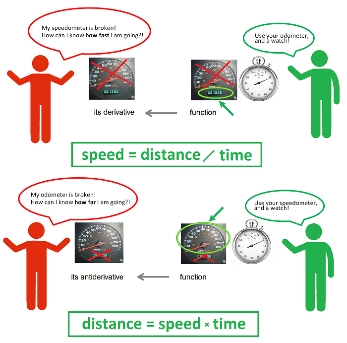
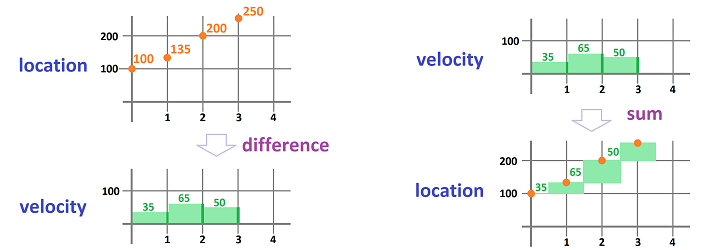
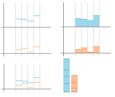
The idea of calculus is presented in a single picture:

The two problems are solved with the help of these two versions of the same elementary school formula: $$\begin{array}{|c|}\hline \quad \text{ speed }= \text{ distance } / \text{ time }\quad \text{ and }\quad \text{ distance }=\text{ speed }\times \text{ time }. \quad \\ \hline\end{array}$$ The formula is solved for the distance or for the speed depending on that is known and what is unknown.

What takes this idea beyond elementary school is the possibility that velocity varies.

Let's be more specific. We consider the same two situations but with more data collected and more information derived from it.

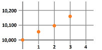
First, imagine that our speedometer is broken. What do we do if we want to estimate how fast we are driving? We look at the odometer several times -- say, every hour on the hour -- during the trip and record the mileage on a piece of paper. The list of our consecutive locations might look like this:

• initial reading: $10,000$ miles;
• after the first hour: $10,055$ miles;
• after the second hour: $10,095$ miles;
• after the third hour: $10,155$ miles;
• etc.

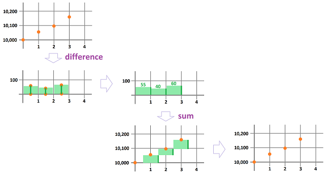
We can plot -- as an illustration -- the locations against time:

But what do we know about the speed? Nothing without algebra! The algebra is simple: $$\text{ speed }= \frac{\text{ distance }}{\text{ time }}.$$ The time interval was chosen to be $1$ hour, so all we need is to find the distance covered during each of these one-hour periods, by subtraction:

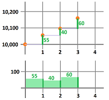
• distance covered during the first hour: $10,055-10,000=55$ miles;
• distance covered during the second hour: $10,095-10,055=40$ miles;
• distance covered during the third hour: $10,155-10,095 =60$ miles;
• etc.

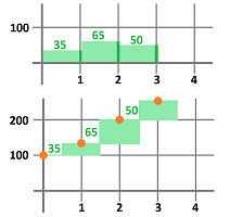
This is how these new numbers appear in the original plot (top):

We also plot these new numbers against time (bottom). As you can see, we illustrate the outcome data in such a way as to suggest that the speed remains constant during each of these hour-long periods.

The problem is solved! We have established that the speed has been -- roughly -- $55$, $40$, and $60$ miles an hour during those three time intervals respectively.

Now on the flip side... Imagine this time that it is the odometer that is broken. If now we want to estimate how far we will have gone, we should look at the speedometer several times -- say, every hour -- during the trip and record its readings on a piece of paper. The result may look like this:

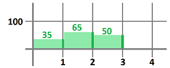
• during the first hour: $35$ miles an hour;
• during the second hour: $65$ miles an hour;
• during the third hour: $50$ miles an hour;
• etc.

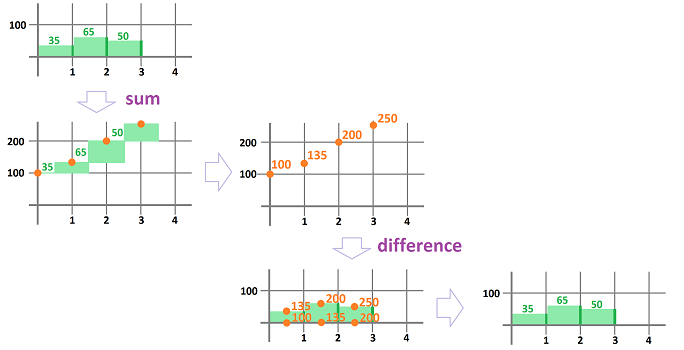
Let's plot our speed against time to visualize that has happened:

Now, what does this tell us about our location? Nothing, without algebra! We use the same formula as before: $$\text{ distance }=\text{ speed }\times \text{ time }.$$ In contrast to the former problem, we need a bit more information though. We must know the starting point of our trip, say, the $100$ mile mark. The time interval was chosen to be $1$ hour, so that we need only to add, and keep adding, the speed at which -- we assume -- we drove during each of these one-hour periods:

• the location after the first hour: $100+35=135$ mile mark;
• the location after the two hours: $135+65=200$ mile mark;
• the location after the three hours: $200+50=250$ mile mark;
• etc.

This is how these new numbers appear in the plot:

The problem is solved! We have established that we have progressed through -- roughly -- $135$, $200$, and $250$ miles marks during this time.

We next consider more complex examples. Here our ability to use negative numbers allows us to treat the data the same way even when we are moving in the opposite direction. As the words “speed” and “distance” suggest their positivity, we speak of the velocity and displacement instead: $$\begin{array}{|c|}\hline \quad \text{ velocity }= \frac{\text{ displacement }}{\text{ time }}\quad \text{ and }\quad \text{ displacement }=\text{ velocity }\cdot \text{ time }. \quad \\ \hline\end{array}$$

First, from location to velocity...

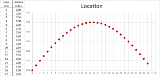
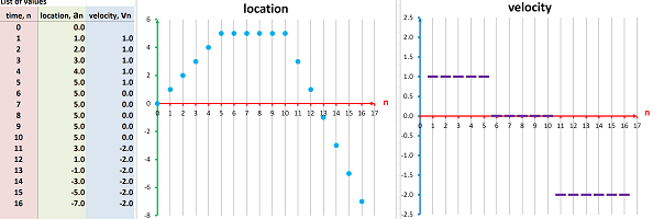
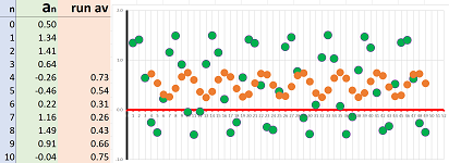
Suppose that this time we have a sequence of more than $30$ data points (more is indicated by “...”); they are the locations of a moving object recorded every minute: $$\begin{array}{l|l|lll} \text{ time } & \text{ min } &0 &1 &2 &3 &4 &5 &6 &7 &8 &9 &10 &...\\ \hline \text{ location } & \text{ miles } & 0.00 &0.10 &0.20 &0.30 &0.39 &0.48 &0.56 &0.64 &0.72 &0.78 &0.84 &...\\ \end{array}$$ This data is seen in the first two columns of the spreadsheet:

Warning: it is entirely a matter of convenience to represent our data as the two-column table in the spreadsheet or the two-row table above it.

The data is furthermore illustrated as a “scatter plot” on the right. It starts to looks like a curve!

Warning: the plot is nothing but a visualization of the data.

To understand how fast we move over these one-minute intervals, we compute the differences of locations for each pair of consecutive locations by pulling data from the previous row. This is how the first one is computed: $$\begin{array}{l|l|ccc} \text{ time } & \text{ min } &0 &1 &...\\ \hline \text{ location } & \text{ miles } & 0.00 &0.10 &...\\ \text{ } & \text{ } & \searrow &\downarrow \\ \text{ difference } & \text{ } & &0.10 -0.00&...\\ \text{ } & \text{ } & &||\\ \text{ velocity } & \text{ miles/min } & &0.10 &...\\ \end{array}$$ We compute these differences for each pair of consecutive locations and then place them in a new row at the bottom of our table: $$\begin{array}{l|l|lll} \text{ time } & \text{ min } &0 &1 &2 &3 &4 &5 &6 &7 &8 &9 &10 &...\\ \hline \text{ location } & \text{ miles } & 0.00 &0.10 &0.20 &0.30 &0.39 &0.48 &0.56 &0.64 &0.72 &0.78 &0.84 &...\\ \text{ } & \text{ } & \searrow &\downarrow &\downarrow &\downarrow &\downarrow &\downarrow &\downarrow &\downarrow &\downarrow &\downarrow &\downarrow &...\\ \text{ velocity } & \text{ miles/min } &- &0.10 &0.10 &0.10 &0.09 &0.09 &0.09 &0.08 &0.07 &0.07 &0.06 &...\\ \end{array}$$

Practically, we prefer to use the spreadsheet. We compute the differences by pulling data from the previous column (locations) with the following formula: $$\texttt{ =RC[-1]-R[-1]C[-1]}.$$ The two values come from the last column, $\texttt{C[-1]}$, same row, $\texttt{R}$, and last row, $\texttt{R[-1]}$, as follows:

We place the result in a new column (velocities):

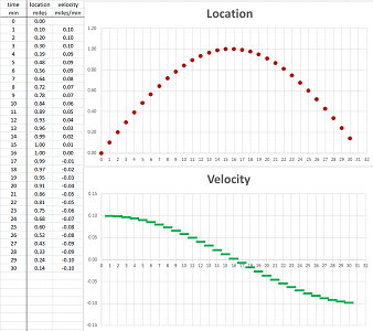
This new data is illustrated with the second scatter plot. To emphasize the fact that the velocity data, unlike the location, is referring to time intervals rather than time instances, we plot it with horizontal segments. In fact, the data table can be rearranged as follows to make this point clearer: $$\begin{array}{l|c|c|c|c|c|c|c|c|c|c} \text{ time } &0 &&1 &&2 &&3 &&4 &&...\\ \hline \text{ location } &0.00 &-&0.10 &-&0.20 &-&0.30 &-& .39&-&...\\ \text{ velocity } &\cdot&0.10& \cdot&0.10& \cdot&0.10& \cdot&0.09& \cdot&0.09 &...\\ \end{array}$$

What has happened to the moving object can now be easily read from the second graph:

• the velocity was positive initially and it was moving in the positive direction;
• it was moving fairly fast but then started to slow down;
• it stopped for a very short period;
• then the velocity became negative as it started to move in the opposite direction;
• it started to speed up in that direction.

Thus, the latter set of data succinctly records some facts about the qualitative and quantitative behavior of the former. As the latter is derived from the former, the transition is described by: $$\begin{array}{|c|}\hline \quad \text{function} \quad \longrightarrow \quad \text{its derivative}. \quad \\ \hline\end{array}$$

Now, from velocity to location...

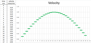
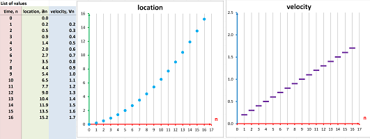
Again, we consider $30$ (or more) data points. These numbers are the values of the velocity of an object recorded every minute: $$\begin{array}{l|l|lll} \text{ time } &\text{ min } &0 &1 &2 &3 &4 &5 &6 &7 &8 &9 &10 &...\\ \hline \text{ velocity }&\text{ miles }&-&0.10 &0.20 &0.30 &0.39 &0.48 &0.56 &0.64 &0.72 &0.78 &0.84 &...\\ \end{array}$$ This data is also seen in the first two columns of the spreadsheet:

The data is furthermore illustrated as a scatter plot on the right. Again, we emphasize the fact that the velocity data is referring to time intervals by plotting its values with horizontal bars.

To find out where we are at the end of each of these one-minute intervals, we compute the sums of velocities (displacements) for each interval by pulling data from the previous row and adding it to the previous result. This is how the first one is computed, under the assumption that the initial location is $0$: $$\begin{array}{l|l|lll} \text{ time } &\text{ min } &0 &1 & ...\\ \hline \text{ velocity }&\text{ miles }&-&0.10 &...\\ \text{ }&\text{ }& &\downarrow&\\ \text{ sum }&\text{ }&0.00 +&0.10 &...\\ \text{ }&\text{ }&\uparrow &|| &\\ \text{ location } &\text{ miles/min } &0.00&0.10 &...\\ \end{array}$$ We place this data in a new row added to the bottom of our table: $$\begin{array}{l|l|lll} \text{ time } &\text{ min } &0 &1 &2 &3 &4 &5 &6 &7 &8 &9 &...\\ \hline \text{ velocity }&\text{ miles }&-&0.10 &0.20 &0.30 &0.39 &0.48 &0.56 &0.64 &0.72 &0.78 &...\\ \text{ } &\text{ } & &\downarrow &\downarrow &\downarrow &\downarrow &\downarrow &\downarrow &\downarrow &\downarrow &\downarrow &...\\ \text{ location } &\text{ miles/min } &0.00 &0.10 &0.30 &0.59 &0.98 &1.46 &2.03 &2.67 &3.39 &4.17 &...\\ \end{array}$$

Practically, we use the spreadsheet. We compute the sums by pulling data from the previous column (velocities) with the following formula: $$\texttt{ =R[-1]C+RC[-1]}.$$ The two values come from the same, $\texttt{C}$, or last, $\texttt{C[-1]}$, column and the same, $\texttt{R}$, and last, $\texttt{R[-1]}$, row, as follows:

We place the result in a new column (locations):

The data is also illustrated as the second scatter plot on the right.

We again rearrange the data table to make the difference between two types of data clearer: $$\begin{array}{l|c|c|c|c|c|c|c|c|c|c} \text{ time } &0 &&1 &&2 &&3 &&4 &&...\\ \hline \text{ velocity } &\cdot&0.00& \cdot&0.10& \cdot&0.20& \cdot&0.30& \cdot&0.39 &...\\ \text{ location } &0.00 &-&0.10 &-&0.30 &-&0.59&-& .98&-&...\\ \end{array}$$

Thus, as the former data set records some facts about the quantitative behavior of the latter, we are able to combine this information to recover the latter. This backward transition is described by: $$\begin{array}{|c|}\hline \quad \text{function} \quad \longrightarrow \quad \text{its antiderivative.} \quad \\ \hline\end{array}$$

This language -- derivatives and antiderivatives -- is justified by the fact that the two operations we have considered undo the effect of each other: $$\text{displacement} \quad \longrightarrow \quad \text{velocity} \quad \longrightarrow \quad \text{same displacement,} $$ and $$\text{velocity} \quad \longrightarrow \quad \text{displacement} \quad \longrightarrow \quad \text{same velocity.} $$

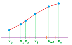
We can further increase the number of data points and, as we zoom out, the scatter plots will look like continuous curves! We now use what we understand about the behavior of the motion data in those tables to describe continuous motion. We simply look at how fast the vertical location is changing relative to the change of the horizontal location:

Furthermore, we replace our time-dependent quantity, location, for another, temperature as a single example of the breadth of applicability of these ideas.

Exercise. Your location is recorded every half-hour, shown below. Estimate your velocity as in terms of time. $$\begin{array}{r|c} \text{time, }x&\text{location, }y\\ \hline 0&20\\ .5&30\\ 1&20\\ 1.5&20\\ 2&50\\ \end{array}$$

The real number line

The starting point of studying numbers is the natural numbers: $$0,1,2,3, ... .$$ They are initially used for counting. The next step is the integers: $$...,-3,-2,-1,0,1,2,3, ....$$ They can be used for studying the space and locations, as follows.

Imagine facing a fence so long that you can't see its ends. We step away from the fence multiple times and there is still more to see:

Is the number of planks infinite? It may be. But for as long as this is convenient, we just assume that we can go on for as long as necessary.

We visualize these as markings on a straight line, according to the order of the planks:

The assumption is that the line and the markings continue without stopping in both directions, which is commonly represented by “$...$”. The same idea applies to the milestones on the road; they are also ordered and might continue indefinitely.

So, we zoomed out to see the fence. Suppose now we zoom in on a location on the fence. What if there is a shorter plank between the two?

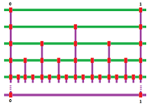
We look closer and we see more... If we keep zooming in, the result will look similar to a ruler:

It's as if we add one mark between two and then repeat this process. We don't have to stop even though this ruler goes only to $1/16$ of an inch.

Is the depth infinite? It may be. But for as long as this is convenient, we just assume that we can go on for as long as necessary.

If we add nine marks at a time, the result is a metric ruler:

Here, we go from meters to decimeters, to centimeters, to millimeters, etc.

To see it another way, we allow more and more decimals in our numbers: $$\begin{array}{rlllllll} 1.55:&1.&1.5&1.55&1.550&1.5500&...;\\ 1/3:&.3&.33&.333&.3333&.33333&...;\\ \pi:&3.&3.1&3.14&3.141&3.1415&.... \end{array}$$

In order to visualize all numbers, we arrange the integers in a line first. The line of numbers is built in several steps.

Step 1: a line is drawn, called an axis, horizontal when convenient:

Step 2: one of the two ends of the line is chosen as positive directions, the one to the right when convenient, then the other is negative:

Step 3: a point $O$ (a letter not number) is chosen as the origin:

Step 4: a segment of the line is chosen as the unit of length:

Step 5: the segment is used to measure distances to locations from the origin $O$ -- positive in the positive direction and negative in the negative direction -- and add marks to the line, the coordinates:

Step 6: the segments are further subdivided to fractions of the unit, etc.:

The end result depends on what the building block is. It may contain gaps and look like a ruler (or a comb) as discussed above. It may also be solid and look like a tile or a domino piece:

So, we start with integers as locations and then -- by cutting these intervals further and further -- also include fractions, i.e., rational numbers. However, we then realize that some of the locations have no counterparts among these numbers. For example, $\sqrt{2}$ is the length of the diagonal of a $1\times 1$ square (and a solution of the equation $x^2=2$); it's not rational. That's how the irrational numbers came into play. Together they form the real numbers.

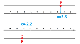
We use this set-up to produce a correspondence between the locations on the line and the real numbers: $$\begin{array}{|c|}\hline \quad \text{location } P\ \longleftrightarrow\ \text{ number } x . \quad \\ \hline\end{array}$$ We will follow this correspondence in both directions, as follows:

• First, suppose $P$ is a location on the line. We then find the nearest mark on the line. That's the “coordinate”, some number $x$, of $P$.
• Conversely, suppose $x$ is a number. We think of it as a “coordinate” and find its mark on the line. That's the location $P$ of $x$ on the line.

Once the coordinate system is in place, it is acceptable to think of every location as a number and vice versa. In fact, we often write: $$P=x.$$

The result may be described as the “$1$-dimensional coordinate system”. It is also called the real number line or simply the number line.

We have created a visual model of the real numbers. Depending on the real number or a collection of numbers that we are trying to visualize, we choose what part of the real line we exhibit; for example, the zero may or may not be in the picture. We also have to choose an appropriate length of the unit segment in order for the numbers to fit in.

In addition to the ruler, another way to visualize numbers is with colors. In fact, in digital imaging the levels of gray are associated with the numbers from $0$ and $255$. A shorter scale -- $1,2, ...,20$ -- can be used (top):

It is also often convenient to associate blue with negative and red with positive numbers (bottom).

Exercise. Think of examples when numbers are visualized with colors.

Sequences

The lists of numbers in the first section are sequences: the locations and the velocities.

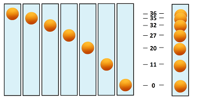
Example (falling ball). We watch a ping-pong ball falling down and recording -- at equal intervals -- how high it is. The result is an ever-expanding string, a sequence, of numbers. If the frames of the video are combined into one image, it will look something like this:

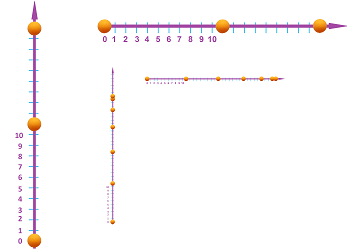
We ignore, for now, the time and concentrate on the locations only. Suppose we have only the first few in a list: $$36,\ 35,\ 32, \ 27,\ 20,\ 11,\ 0.$$ This data can be visualized by placing the ball at every coordinate location on the real line, vertically or horizontally:

Though not uncommon, this method of visualization of motion, or of sequences in general, has its drawbacks: overlapping may be inevitable and the order of events is lost without labels. A more popular approach is the following. The idea is to separate time and space, give a separate real line, an axis, to each moment of time, and then bring them back together in one rectangular plot:

The location varies -- as it does -- vertically while the time progresses horizontally. The result is similar to the collection of the frames of the video as seen above. The plot is called the graph of the sequence.

As far as the data is concerned, we have a list of pairs, time and location, arranged in a table: $$\begin{array}{r|ll} \text{moment}&\text{height}\\ \hline 1&36\\ 2&35\\ 3&32\\ 4&27\\ 5&20\\ 6&11\\ 7&0 \end{array}$$ The table is just as effective representation of the data if we flip it; it's more compact: $$\begin{array}{l|ll} \text{moment:}&1&2&3&4&5&6&7\\ \hline \text{height:}&36&35&32&27&20&11&0 \end{array}$$ This transformation is called the transposition. $\square$

So, it is the most common way to visualize sequences of numbers as sequences of points on a sequence of vertical axes:

It is also common to represent the same numbers as vertical bars:

Warning: the graph is just a visualization.

To represent a sequence algebraically, we first give it a name, say, $a$, and then assign a special variation of this name to each term of the sequence: $$\begin{array}{ll|ll} \text{index:}&n&1&2&3&4&5&6&7&...\\ \hline \text{term:}&a_n&a_1&a_2&a_3&a_4&a_5&a_6&a_7&... \end{array}$$ The subscript is called the index; it indicates the place of the term within the sequence. We say “$a$ sub $1$”, “$a$ sub $2$,” etc. Just as before, “...” indicates a continuing pattern.

Example (falling ball). In the last example, we name the sequence $h$ for “height”. Then the above table take this form: $$\begin{array}{l|ll} \text{moment:}&1&2&3&4&5&6&7&...\\ \hline \text{height:}&h_1&h_2&h_3&h_4&h_5&h_6&h_7&...\\ &||&||&||&||&||&||&||&...\\ \text{height:}&36&35&32&27&20&11&0&... \end{array}$$ When abbreviated, it takes the form of this list: $$h_1=36,\ h_2=35,\ h_3=32, \ h_4=27,\ h_5=20,\ h_6=11,\ h_7=0.$$ $\square$

So, we use the following notation: $$a_1=1,\ a_2=1/2,\ a_3=1/3,\ a_4=1/4,\ ...,$$ where $a$ is the name of the sequence and adding a subscript indicates which term of the sequence we are facing.

A sequence can come from a list or a table unless it's infinite. Infinite sequences often come from formulas.

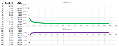
Example (reciprocals). The formula: $$a_n=1/n,$$ gives rise to the sequence, $$a_1=1,\ a_2=1/2,\ a_3=1/3,\ a_4=1/4,\ ....$$ Indeed, replacing $n$ in the formula with $1$, then $2$, $3$, etc. produces the numbers on the list one by one, as follows. We enter $n$ into the formula and $a_n$ appears at the end of the computation. In other words, we place the current value of $n$ inside a blank box (where $n$ used to be) in the formula: $$\begin{array}{ccrlccc} &&\Large{a}_\square &&=&\frac{1}{\square }\\ &&\uparrow&&&\uparrow\\ &&\text{ insert }n&&&\text{insert }n \end{array}$$ It is called “substitution”. We do this seven times below: $$\begin{array}{l|ll} n:&1&2&3&4&5&6&7&...\\ \hline a_n:&a_1&a_2&a_3&a_4&a_5&a_6&a_7&...\\ &||&||&||&||&||&||&||&...\\ \frac{1}{n}&\frac{1}{1}&\frac{1}{2}&\frac{1}{3}&\frac{1}{4}&\frac{1}{5}&\frac{1}{6}&\frac{1}{7}&... \end{array}$$ With a formula, we can use a spreadsheet to produce more values as well as plot them:

The complete representation is as follows: $$a_n=1/n,\ n=1,2,3, ...$$ $\square$

Exercise. Write a few terms of the sequences given by the formulas:

• (a) $a_n=3n-1$;
• (b) $b_n=1+\frac{1}{n}$.

Thus, every formula is capable of creating an infinite sequence $a_n$. For example, we can take

• $a_n=n$,
• $b_n=n^2$,
• $c_n=n^3$,
• etc.

This is a whole class of sequences.

Definition. For every positive integer $p$, a power sequence, or a $p$-sequence, is given by the formula: $$a_n=n^p, \quad n=1,2,3,....$$

The relation between the sequences becomes clear if we zoom out on their graphs:

Indeed, the larger the power $p$, the faster the sequence grows. The relation between the consecutive terms of each sequence is also clear: growth! We use this word when we see the graph that rises but it can also drop (seen zoomed out):

As you can see, the behavior varies even within these two categories: increasing and decreasing.

The precise definition has to rely on considering every pair of consecutive terms of the sequence. For example, our sequence, $36,\ 35,\ 32, \ 27,\ 20,\ 11,\ 0$, is decreasing because: $$36> 35> 32> 27> 20> 11> 0.$$

Definition. A sequence $a_n$ is called increasing if, for all $n$, we have: $$a_n\le a_{n+1};$$ It is called decreasing if, for all $n$, we have: $$a_n\ge a_{n+1};$$ collectively they are called monotone.

Warning: both increasing and decreasing sequences may have segments with no change; furthermore, a constant sequence is both increasing and decreasing.

Example (monotone). When the sequence is given by its formula, we use it directly. The sequence $a_n=n^2$ is proven to be increasing by making the following connection:

• we know that $n<n+1$, therefore $n^2<(n+1)^2$.

An abbreviated way to write this is as follows. For every $n=1,2,3...$, we have: $$n<n+1\ \Longrightarrow\ n^2<(n+1)^2.$$ Similarly, $\frac{1}{n}$ is decreasing: $$n<n+1\ \Longrightarrow\ \frac{1}{n}<\frac{1}{n+1}.$$ The sequence $$1,-1,1,-1,1,-1,1,-1,1,-1,....$$ is neither increasing nor decreasing, i.e., it's not monotone. $\square$

Exercise. Show that $\frac{1}{2^{n}}$ is decreasing

Exercise. Show that all power sequences increase.

A major reason why we study sequences is that their terms can often be defined in a consecutive manner.

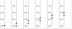
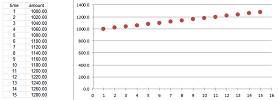
Example (regular deposits). A person starts to deposit $\$20$ every month to in his bank account that already contains $\$ 1000$. Then, after the first month the account contains: $$ \$1000+\$20=\$ 1020,$$ after the second: $$ \$1020+\$20=\$ 1040,$$ and so on. Then, if $a_n$ is the amount in the bank account after $n$ months, we have a formula: $$a_{n+1}=a_n+ 20.$$ How much will I have after $50$ years? I'd have to carry out $50\cdot 12$ additions... For the spreadsheet, the formula is: $$\texttt{=R[-1]C+20}.$$ Below, the current amount is shown in blue and the next -- computed from the current -- is shown in red:

Plotting the whole sequence at once confirms that the sequence is increasing:

It looks like a straight line... $\square$

Thus, in addition to tables and formulas, a sequence can be defined by computing its terms consecutively, one at a time. We say that a sequence $a_n$ is recursive when its next term is found from the current term (or several previous terms) by a formula.

Definition. A sequence defined (recursively) by the formula: $$a_{n+1}=a_n+ b,$$ is called an arithmetic progression with $b$ its increment.

Exercise. If the increment is zero, the sequence is...

Example (compounded interest). An arithmetic progression is repetitive... Also repetitive is the following typical situation. A person deposits $\$ 1000$ in his bank account that pays $1\%$ APR compounded annually. Then, after the first year, the interest is $$ \$1000\cdot.01=\$ 10,$$ and the total amount becomes $\$1010$. After the second year we have the interest: $$ \$1010\cdot .01=\$ 10.10,$$ and so on. In other words, the total amount is multiplied by $.01$ at the end of each year and then added to the total. An even simpler way to put this is to say that the total amount is multiplied by $1.01$ at the end of each year, as follows. Then, after the first year, the interest is $$ \$1000\cdot 1.01=\$ 1010,$$ and the total amount becomes $\$1010$. After the second year we have the interest: $$ \$1010\cdot 1.01=\$ 1020.1,$$ and so on. Putting this together, let $a_n$ represent the amount in the bank account after $n$ years, then we have a recursive formula: $$a_{n+1}=a_n\cdot 1.01.$$ How much will I have after $50$ years? I'd have to carry out $50$ multiplications... For the spreadsheet, the formula is: $$\texttt{=R[-1]C*1.01}.$$

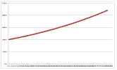
Only after repeating the step $100$ times one can see that this isn't just a straight line:

The sequence is increasing. $\square$

Definition. A sequence defined (recursively) by the formula: $$a_{n+1}=a_n\cdot r,$$ with $r\ne 0$, is called a geometric progression with $r$ its ratio. We say that this is

• geometric growth when $r>1$, and
• geometric decay when $r<1$.

Alternatively, it is called exponential growth and decay respectively.

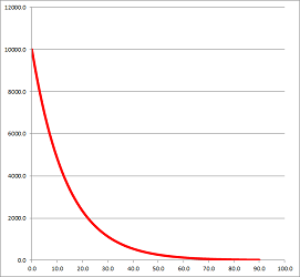
Example (population loss). If the population of a city declines by $3\%$ every year, it is left with $97\%$ of its population at the end of each year. The result is found by multiplying by $.97$, every time. We have, therefore: $$\overbrace{( \underbrace{\underbrace{(1,000,000 \cdot 0.97 )}_{\textrm{after 1 year}} \cdot 0.97}_{\textrm{after 2 years}} ) \cdot 0.97}^{\textrm{after 3 years}}.$$ And so on. What will be the population after $50$ years? I'd have to carry out $50$ multiplications... The long term pattern is clear from the graph:

This is a geometric progression with ratio $r=.97$, i.e., geometric decay. The sequence is decreasing and eventually there is almost nothing left... $\square$

Example (saving). What if we deposit money to our bank account and receive interest? The recursive formula is simple, for example: $$a_{n+1}=a_n\cdot 1.05+200.$$ $\square$

When a sequence is defined recursively, we'd need to carry out this definition $n$ times in order to find the $n$th term... This is in contrast to sequences defined directly via its $n$th term formula, such as $a_n=n^2$, that require a single computation.

Below, we keep multiplying, just as in the geometric progression, but this time the multiple grows...

Definition. The factorial is the sequence defined (recursively) as follows: $$a_0=1,\quad a_n=a_{n-1}\cdot n,\ n\ge 1;$$ i.e., we have for $n=1,2,3...$: $$a_n=1\cdot 2 \cdot ... \cdot (n-1)\cdot n ,$$ denoted by $$n!=1\cdot 2 \cdot ... \cdot (n-1)\cdot n.$$

For example, this is how a few initial terms are computed. We progress from left to right in the bottom row by following the arrow $\nearrow$ to find and multiply by the current value of $n$, then placing the result where the next arrow $\downarrow$ points: $$\begin{array}{r|ll} n&0&&1&&2&&3&&4&...\\ &&\nearrow&\downarrow&\nearrow&\downarrow&\nearrow&\downarrow&\nearrow&\downarrow&...\\ a_n=n!&1&&1&&2&&6&&24&... \end{array}$$

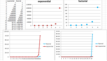
The factorial exhibits a very fast growth, eventually:

You can see how it stays behind the geometric progression with ratio $r=10$ but then leaps ahead.

The factorial appears frequently in calculus and elsewhere. It suffices to point out for now that it counts in how many ways one can permute objects. We notice that it is about placing $n$ objects into $n$ slots, one by one:

• the first object has $n$ options,
• the second $n-1$ options,
• the third $n-2$ options,
• ...
• the last has $1$ option.

Since the choices are independent of each other, the total number of such placements is $n(n-1)\cdot ...2\cdot 1=n!$.

We say $n$-factorial to refer to the $n$th term of this sequence, $n!$.

THEOREM. The number of all possible permutations of $n$ objects is equal to $n$-factorial.

Exercise. In how many ways can you arrange $9$ players at the $9$ positions on the baseball field?

Warning: $n!$ is just an abbreviation of the recursive definition of the factorial, not its $n$th term formula.

Repeated addition and repeated multiplication

In this section, we will take a better look at the arithmetic and geometric progressions, side by side.

Remember this simple algebra:

• repeated addition is multiplication: $2 + 2 + 2 = 2 \cdot 3$.

One can say that that's how multiplication was “invented” -- as repeated addition. What about repeated multiplication?

• repeated multiplication is power: $2 \cdot 2 \cdot 2 = 2^{3}$.

In other words, we prefer to have an abbreviated notation for repetitive operations.

That's why -- in addition to the recursive formulas -- we have $n$th term formulas for these sequences:

• (1) the $n$th-term formula for an arithmetic progression with increment $b$ and initial term $a_0$ is:

$$a_{n}=a_0+ b\cdot n,\ n=1,2,3...$$

• (2) the $n$th-term formula for a geometric progression with ratio $r$ and initial term $a_0$ is:

$$a_{n}=a_0\cdot r^n,\ n=1,2,3...$$

So, we face two similar conventions of algebra:

• a real number $a$ added to itself $n$ times is replaced with $a\cdot n$; while
• a real number $a$ multiplied by itself $n$ times is replaced with $a^n$.

Recall the notation and the terminology for the latter: $$\begin{array}{rl} &\text{exponent}\\ &\downarrow\\ &\small{n}\\ \Large{a}\\ \uparrow\\ \text{base} \end{array}$$

We will pursue this big analogy further and re-discover some familiar algebraic properties. This is entirely about counting how many times you carry out the operation: adding $a$ or multiplying by $a$.

The first set of properties is about the algebraic operations carried out with the values of two sequences (repetitions in parallel). $$\begin{array}{r|rl|rl} n=1,2,3, ...&\text{repeated addition}&=\text{multiplication}&\text{repeated multiplication}&=\text{power}\\ \hline \text{Convention:}&\underbrace{a+a+a+...+a}_{n\text{ times}}&=a\cdot n&\underbrace{a\cdot a\cdot a\cdot ...\cdot a}_{n\text{ times}}&=a^n\\ \hline \text{Repeated }n \text{ times,}&\underbrace{a+a+a+...+a}_{n\text{ times}}\qquad&=a\cdot n&\underbrace{a\cdot a\cdot a\cdot ...\cdot a}_{n\text{ times}}\qquad&=a^n\\ \text{then }m \text{ times more.}&\qquad+\underbrace{a+a+a+...+a}_{m\text{ times}}&\quad=a\cdot m&\qquad\cdot \underbrace{a\cdot a\cdot a\cdot ...\cdot a}_{m\text{ times}}&\quad=a^m\\ \text{Count:}&\underbrace{\quad\qquad\qquad\qquad\qquad}_{n+m\text{ times}}&&\underbrace{\qquad\qquad\qquad}_{n+m\text{ times}}&\\ \hline \text{Property 1:}&a\cdot (n+m)&=a\cdot n+a\cdot m & a^{n+m}&=a^n\cdot a^m\\ \hline \end{array}$$

This property for addition, $$a\cdot (n+m)=a\cdot n+a\cdot m,$$ is called the Distributive Property. It “distributes” multiplication over addition and undoes the effect of factoring.

Warning: we don't “distribute” exponentiation over addition: $a^{n+m} \ne a^n+ a^m$.

Warning: we also can't “distribute” exponentiation over addition this way: $(a+b)^n \ne a^n+b^n$.

The second set of properties is also about the algebraic operations carried out with the values of the sequences. $$\begin{array}{r|rl|rl} n=1,2,3, ...&\text{repeated addition}&=\text{multiplication}&\text{repeated multiplication}&=\text{power}\\ \hline \text{Convention:}&\underbrace{a+a+a+...+a}_{n\text{ times}}&=a\cdot n&\underbrace{a\cdot a\cdot a\cdot ...\cdot a}_{n\text{ times}}&=a^n\\ \hline \text{Repeated }n \text{ times.}&\underbrace{a+a+a+...+a}_{n\text{ times}}&=a\cdot n&\underbrace{a\cdot a\cdot a\cdot ...\cdot a}_{n\text{ times}}&=a^n\\ \text{Repeated }n \text{ times.}&+\underbrace{b+b+b+...+b}_{n\text{ times}}&=b\cdot n&\cdot \underbrace{b\cdot b\cdot b\cdot ...\cdot b}_{n\text{ times}}&=b^n\\ \text{Count:}&=\underbrace{(a+b)+...+(a+b)}_{n\text{ times}}&&=\underbrace{(a\cdot b)\cdot ...\cdot (a\cdot b)}_{n\text{ times}}&\\ \hline \text{Property 2:}&(a+b)\cdot n&=a\cdot n+b\cdot n & (a\cdot b)^n &=a^n\cdot b^n\\ \hline \end{array}$$

This property for addition, $$(a+b)\cdot n=a\cdot n+b\cdot n,$$ is, once again, the Distributive Property. It “distributes” multiplication over addition. The corresponding property for multiplication, $$(a\cdot b)^n =a^n\cdot b^n,$$ “distributes” exponentiation over multiplication.

In contrast to the properties above, the next set is about compositions (repeat the repeated). $$\begin{array}{r|c|rl|rl} n=1,2,3, ...&&\text{repeated addition}&=\text{multiplication}&\text{repeated multiplication}&=\text{power}\\ \hline \text{Convention:}&&\underbrace{a+a+a+...+a}_{n\text{ times}}&=a\cdot n&\underbrace{a\cdot a\cdot a\cdot ...\cdot a}_{n\text{ times}}&=a^n\\ \hline \text{Repeated }n \text{ times,}&1.&\underbrace{a+a+a+...+a}_{n\text{ times}}&=a\cdot n& \underbrace{a\cdot a\cdot a\cdot ...\cdot a}_{n\text{ times}}&=a^n\\ m \text{ times.}&2.&+\underbrace{a+a+a+...+a}_{n\text{ times}}&=a\cdot n&\cdot\underbrace{a\cdot a\cdot a\cdot ...\cdot a}_{n\text{ times}}&=a^n\\ &\vdots&\vdots\qquad&\quad\vdots&\vdots\quad&\quad\vdots\\ &m.&+\underbrace{a+a+a+...+a}_{n\text{ times}}&=a\cdot n&\cdot\underbrace{a\cdot a\cdot a\cdot ...\cdot a}_{n\text{ times}}&=a^n\\ \text{Count:}&&\underbrace{\quad\qquad\qquad\qquad\qquad}_{nm\text{ times}}&\ \ \underbrace{\quad}_{m\text{ times}}&\underbrace{\quad\qquad\qquad\qquad}_{nm\text{ times}}&\ \ \underbrace{\quad}_{m\text{ times}}\\ \hline \text{Property 3:}&&a\cdot(n\cdot m)&=(a\cdot n)\cdot m & a^{n\cdot m}&=(a^n)^m\\ \hline \end{array}$$

The third property for addition, $$a\cdot(n\cdot m)=(a\cdot n)\cdot m,$$ is called the Associativity Property of addition. It means that multiplications can be re-grouped (the middle number can be “associated” with the last one or the next one) arbitrarily. The corresponding property for multiplication, $$a^{(n\cdot m)}=(a^n)^m,$$ means that exponentiations can be re-grouped arbitrarily too.

Example. These properties/rules operate as shortcuts. First, $$2^{3} \cdot 2^{2} = 2^{3}\cdot 2^{2} = 2^{3+2} = 2^{5};$$ second, $$(2\cdot 3)^5=2^5\cdot 3^5;$$ third, $$ (2^{3})^{4} = 2^{3\cdot 4} = 2^{12}.$$ However, when read from right to left, these properties serve as decompositions. $\square$

Exercise. Simplify: $$5^{0} \cdot 5^{3},\ (4\cdot 3)^2,\ (3^{3})^{3},\ 1^{3+3},\ 5^1\cdot 3^1,\ 2^{2\cdot 2} .$$

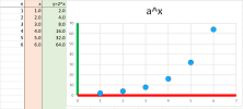
So far, we are facing nothing but a geometric progression with ratio $a$:

What about $0$? But what would be the outcome -- and the meaning -- of repeating an algebraic operation zero times? We will need another convention!

We know what it is for addition; we choose: $$\begin{array}{|c|}\hline \quad a\cdot 0=0. \quad \\ \hline\end{array}$$ For multiplication, we choose, for $a\ne 0$: $$\begin{array}{|c|}\hline \quad a^0=1. \quad \\ \hline\end{array}$$ But why? Why not $0$? Why not any other number? Because we want the three properties still to be satisfied! This way we can continue to use them as if nothing has changed.

Let's check. We plug in $n=0$ or $m=0$ and use our convention: $$\begin{array}{r|ll|ll} \text{Property 1:} & a^{n+m} &=a^n\cdot a^m & n=0 & \Longrightarrow & a^{0+m}&=a^0\cdot a^m & \Longleftrightarrow & a^m=1\cdot a^m & \texttt{TRUE!}\\ \hline \text{Property 2:} & a^n b^n &=(ab)^n & n=0 & \Longrightarrow & a^0 b^0 &=(ab)^0 & \Longleftrightarrow & 1\cdot 1=1 & \texttt{TRUE!}\\ \hline \text{Property 3:} & a^{nm} &=(a^n)^m & n=0 & \Longrightarrow & a^{0m} &=(a^0) ^m & \Longleftrightarrow & a^0=1^m & \texttt{TRUE!}\\ & && m=0 & \Longrightarrow & a^{n0} &=(a^n)^0 & \Longleftrightarrow & a^0=1 & \texttt{TRUE!}\\ \end{array}$$ The three properties are still satisfied, and we will continue to use them. Note how choose anything but $a^0=1$ would have ruined them.

From now on, the formula for geometric progression, $$a_n=ar^n,$$ can start with a zeroth term.

In particular, the compounded interest sequence will start with the initial deposit, $a_0$.

This is the summary of the algebra of exponents ($a$ and $b$ any real numbers): $$\begin{array}{r|rl|rl} \text{}&\text{Multiplication:}&&\text{Exponentiation:}\\ \hline n=1,2,3, ...&\underbrace{a+a+a+...+a}_{n\text{ times}}&=a\cdot n&\underbrace{a\cdot a\cdot a\cdot ...\cdot a}_{n\text{ times}}&=a^n\\ n=0 & a\cdot 0 & =0 & a^0&=1\\ \hline \text{Rules: } 1.&a\cdot (n+m)&=a\cdot n+a\cdot m & a^{n+m}&=a^n\cdot a^m\\ \hline 2.&(a+b)\cdot n&=a\cdot n+b\cdot n & (a\cdot b)^n&=a^n\cdot b^n\\ \hline 3.&a\cdot(n\cdot m)&=(a\cdot n)\cdot m & a^{n\cdot m}&=(a^n)^m\\ \hline \end{array}$$ Note that the right-hand sides of the rules are matched: just replace “$+$” with “$\cdot$” and “$\cdot$” with “$^\wedge $” in the first column and you get those in the second. For example, this is how Rule 1 works: $$\begin{array}{ccc} a&\cdot &(n+m)&=&a&\cdot& n&+&a&\cdot &m \\ a&^\wedge &(n+m)&=&a&^\wedge &n&\cdot& a&^\wedge &m\\ \end{array}$$ The two rules are truly parallel. However, this is not the case -- warning! -- for the left-hand sides of the rules. The reason is that some of the algebra in the left-hand sides has come from counting the repetitions, identically for both columns.

We will further continue to expand the idea of exponent in Chapter 4.

A related convention is the following: $$\begin{array}{|c|}\hline \quad 0!=1. \quad \\ \hline\end{array}$$

How to find $n$th term formulas for sequences

Using the algebra discussed in the last section allows us to produce explicit formulas. First, for an arithmetic progression, we have a recursive formula: $$a_{n+1}=a_n+b.$$ Written explicitly, it takes this form: $$a_n=a_0+\underbrace{b+b+b+...+b}_{n\text{ times}}.$$ Finally, we have another representation now, without “...”!

THEOREM (Arithmetic progression). The $n$th-term formula for an arithmetic progression with increment $b$ and initial term $a_0$ is: $$a_{n}=a_0+ b\cdot n,\quad n=0,1,2,3...$$

Second, for a geometric progression, we have a recursive formula: $$a_{n+1}=a_n\cdot r.$$ Written explicitly, it takes this form: $$a_n=a_0\cdot\underbrace{r\cdot r\cdot r\cdot ...\cdot r }_{n\text{ times}}.$$ Finally, we have another representation now, without “...”!

THEOREM (Geometric progression). The $n$th-term formula for a geometric progression with ratio $r$ and initial term $a_0$ is: $$a_{n}=a_0\cdot r^n,\quad n=0,1,2,3...$$

For these two sequences, given originally by their recursive formulas, are now presented by their $n$-th term formulas.

It is also sometimes possible, starting with a list, work your way backwards and invent such a formula.

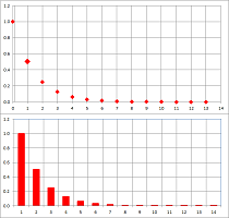
Example. What is the formula for this sequence: $$1,\ 1/2,\ 1/4,\ 1/8,\ ...?$$ First, we notice that the numerators are just $1$s: $$\frac{1}{1},\ \frac{1}{2},\ \frac{1}{4},\ \frac{1}{8} ...$$ Second, the denominator is multiplied by $2$ every time. It is the same as to multiply the whole fraction by $\frac{1}{2}$. The recursive formula is then: $$a_{n+1}=a_n\cdot \frac{1}{2}.$$ It is a geometric progression! Its ratio is $r=a/2$ and its initial term is $a_0=1$. According to the theorem, we have $$a_n=1\cdot\left(\frac{1}{2}\right)^{n}=\frac{1}{2^{n}}.$$ If the pattern in clear from the beginning, we skip the recursive state and just observe that the denominators are the powers of $2$: $$a_0=1,\ a_1=\frac{1}{2},\ a_2=\frac{1}{2^2},\ a_3=\frac{1}{2^3},\ ....$$ and then derive the formula directly. With this formula, we can plot more terms:

$\square$

Exercise. What is the formula for the sequence if it starts with $a_1=1$ instead?

Example (alternating). What is the formula for this sequence: $$1,\ -1,\ 1,\ -1,\ ...?$$

First, we notice that the absolute values of these numbers are just $1$s and while the sign alternates. We write it in a more convenient form: $$a_0=1,\ a_1=-1,\ a_2=1,\ a_3=-1,\ ....$$ The pattern in clear and the correspondence can be written for the two cases: $$a_n=\begin{cases} -1&\text{ if } n \text{ is even},\\ 1&\text{ if } n \text{ is odd}. \end{cases}$$ This qualifies as its $n$th term formula but there is a more compact version: $$a_n=(-1)^{n}.$$ We were able to get rid of “...”! $\square$

Exercise. What is the formula for the sequence if it starts with $a_1=1$ instead?

Exercise. The alternating sequence above is a ________ sequence.

Exercise. Point out a pattern in each of the following sequences and suggest a formula for its $n$th term whenever possible:

• (a) $1,\ 3,\ 5,\ 7,\ 9,\ 11,\ 13,\ 15,\ ...$;
• (b) $.9,\ .99,\ .999,\ .9999,\ ...$;
• (c) $1/2,\ -1/4,\ 1/8,\ -1/16,\ ...$;
• (d) $1,\ 1/2,\ 1/3,\ 1/4,\ ...$;
• (e) $1,\ 1/2,\ 1/4\ ,1/8,\ ...$;
• (f) $2,\ 3,\ 5,\ 7,\ 11,\ 13,\ 17,\ ...$;
• (g) $1,\ -4,\ 9,\ -16,\ 25,\ ...$;
• (h) $3,\ 1,\ 4,\ 1,\ 5,\ 1,\ 9,\ ...$.

Example (regular deposits). A person starts to deposit $\$20$ every month to in his bank account that already contains $\$ 1000$: $$a_{n+1}=a_n+ 20.$$ We have now a formula for the $n$th term: $$a_{n}=1000+ 20\cdot n,$$ assuming that $a_0=1000$.

$\square$

Exercise. How long will it take to double your money?

Example (compounded interest). A person deposits $\$ 1000$ in his bank account: $$a_{n+1}=a_n\cdot 1.01.$$ We have now a formula: $$a_{n+1}=1000\cdot 1.01^n.$$

This is the general setup. A person deposits $a_0$ dollars to his bank account. Suppose the account pays $R$, the decimal representation of the APR compounded annually, i.e., $.10$ for $10$ percent etc. The total amount is then multiplied by $1+R$ at the end of each year and then added to the total. Now if $a_n$ stands for the amount in the bank account after $n$ years, we have the following recursive formula: $$a_{n+1}=a_n\cdot (1+R).$$ A verbal description of the model: the growth is proportional to the size of current amount reveals that this is a geometric progression. This is just a geometric progression and its $n$th-term formula is: $$a_n=a_0\cdot (1+R)^n, n=1,2,3...$$ $\square$

Exercise. How long will it take to double your money?

Example (bacteria multiplying). Suppose we have a population of bacteria that doubles every day. For example, we can imagine that every one of them divides in half every day. Let $p_n$ be the number of bacteria after $n$ days: $$\underbrace{p_{n+1}}_{\text{population: at time } n+1} = \underbrace{2p_n}_{\text{ at time } n}.$$ To know $p_n$ for all $n$, we need to know the initial population $p_0$.

A verbal description of the model: the growth is proportional to the size of population reveals that this is a geometric progression. We already have an $n$th term formula: $$p_n = p_0 2^{n}. $$ $\square$

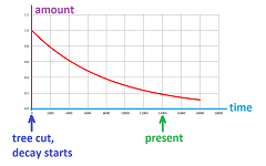
Example (radioactive decay and radiocarbon dating). It is known that, once the tree is cut, the radioactive carbon it contains starts to decay. It loses half of its mass over a certain period of time called the half-life of the element. The loss, therefore, follows the familiar exponential decay model: $$a_{n+1}=a_n\cdot \frac{1}{2}.$$ A verbal description of the model: the decay is proportional to the current amount reveals that this is a geometric progression. The difficulty is that here $n$ is not the number of years but the number of half-lives! For example, the percentage of this element, $^{14}\text{C}$, left is plotted below:

The idea we will develop is as follows:

• know the element's half-life;
• measure the percentage of the element present vs. the amount normally present;
• calculate the time when tree was cut.

Suppose the half-life is $5730$ years (i.e., the time it takes to go from $100\%$ to $50\%$). Parchment has $74\%$ of $^{14}\text{C}$ left. How old is it?

Unfortunately, the model measures time in a multiples of the half-life, $5730$ years. Any period shorter than that is out reach for now. We can try to estimate the answer by assuming that this is a arithmetic progression, yearly:

The period is therefore is estimated to be close to: $$\frac{1}{4}\text{-life} = \frac{1}{2}\left( \frac{1}{2}\text{-life} \right)= 2865.$$ We will learn how to deal with fractional period and solve the problem exactly in Chapter 4. $\square$

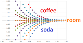
Example (Newton's Law of Cooling). The dynamics of cooling of an object is depends on the difference between its temperature $T_n$ and the room temperature $R$. This number determines the new temperature $T_{n+1}$. The law states that the rate of cooling is proportional to this difference: $$T_{n+1}-R=(T_n-R)\cdot k,$$ for some $k<1$. We, therefore, have a recursive formula: $$T_{n+1}=R+(T_n-R)\cdot k.$$ Unless $R=0$, this is not a geometric progression (but $T_n-R$ is). We plot below several sequences for the two cases: $T_0 > R$ (cooling) and $T_0<R$ (warming):

$\square$

Exercise. Find the $n$th term formula for the sequence in the above example.

Collectively, these examples are called exponential models: the growth is proportional to the current term. There are other types.

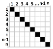
Example (round robin). If we have $n$ teams to play each other exactly once, how many games do we have to plan for? A table commonly used for such a tournament is below:

The table reveals the following. The first team is to play $n-1$ games. The second also is to play $n-1$ games but one less is actually counted as it is already on the first list. The third is to play $n-1$ games but two less is actually counted as they are already on the first and second lists. And so on. The total is: $$(n-1)+(n-2)+...+2+1.$$ We can treat this as a recursive sequence: $$a_1=1,\ a_{n+1}=a_n+n.$$ How do we find an explicit, direct formula for the $n$th term of this sequence? The table tells us the answer. The total number of cells in the table is $n^2$. Without the diagonal ones, it's $n^2-n$. Finally, we take only half of those: $(n^2-n)/2$. As a purely mathematical conclusion, the sum of $n$ consecutive integers starting from $1$ is the following: $$1+2+3+...+n=\frac{n(n+1)}{2}.$$ We were able to get rid of “...”! $\square$

Exercise. Show that the sum of consecutive odd numbers satisfies the following: $$1+3+5+7+... +(2n-1)=n^2.$$

Can we always find an explicit formula? No. We have already seen an example of a recursively defined sequence without $n$th term formula, the factorial, $n!$.

Example. What if we deposit money to our bank account and receive interest? The recursive formula is simple, for example: $$a_{n+1}=a_n\cdot 1.05+200.$$ Is there a direct formula? It's too cumbersome to be of any use: $$a_n=\bigg(...\big((a_0\cdot 1.05+200)\cdot 1.05+200\big)..._\text{ repeat n times }\bigg)\cdot 1.05+200.$$ Since we don't know how to get rid of “...”, we are left with a formula which is just the recursive definition of the sequence in disguise. Best we can tell is that the sequence is increasing. $\square$

Example (restricted growth). Suppose our bacteria live in a jar. We are then forced to add another effect to our population model:

• the rate of reproduction will still be proportional to the current population -- but only when the population size is “small”; and
• once it's “large”, starvation starts -- the growth rate will decrease at a rate proportional to how close is the population to the theoretical carrying capacity.

For example, suppose, in the case of bacteria, the jar can accommodate $1000$. Then the recursive formula $p_{n+1}=2p_n$ is modified by adding a new factor: $$p_{n+1}=2p_n\cdot \frac{1000-p_n}{1000}.$$ For example, if the current population is $p_n=800$, the next is $$p_{n+1}=2\cdot 800\cdot \frac{1000-800}{1000}=320.$$ It goes down because it was too close to the capacity. But the next one, $$p_{n+2}=2\cdot 320\cdot \frac{1000-320}{1000}=435.2 $$ is up again! In general, we define a sequence to represent the proportion of the largest possible population: $$a_{n+1}=ra_n(1-a_n),$$ where $r>0$ is a parameter. For the spreadsheet, the formula is: $$\texttt{=R2C2*R[-1]C*(1-R[-1]C)},$$ where $\texttt{R2C2}$ is the cell that contains the value of $r$. For example, this is what we have for $r=3.9$ (and $a_1=.5$):

Such a sequence is called a logistic sequence. Its dynamics dramatically depends on $r$:

Above, the sequence starts with $1/2$ value and then shows the following dynamics: decay, constant, oscillating convergence, and chaos. There is no $n$th term formula. $\square$

Exercise. What if new bacteria are introduced to the jar at a constant rate?

The algebra of exponents

Recall our analysis from earlier on where the exponents -- by analogy with multiplication -- come from: $$\begin{array}{r|rl|rl} \text{}&\text{Multiplication:}&&\text{Exponentiation:}\\ \hline n=1,2,3, ... &\underbrace{a+a+a+ ... +a}_{n\text{ times}}&=a\cdot n&\underbrace{a\cdot a\cdot a\cdot ... \cdot a}_{n\text{ times}}&=a^n\\ n=0 & a\cdot 0 & =0 & a^0&=1\\ \hline \text{Rules: } 1.&a(n+m)&=a\cdot n+a\cdot m & a^{n+m}&=a^n\cdot a^m\\ \hline 2.&(a+b)n&=a\cdot n+b\cdot n & (ab)^n&=a^n b^n\\ \hline 3.&a\cdot(nm)&=(a\cdot n)\cdot m & a^{nm}&=(a^n)^m\\ \hline \end{array}$$

Exercise. Represent as a power of $3$: $$3^3\cdot 9.$$

Let's review what we know about factoring integers: $$\begin{array}{|l|} \hline \text{A prime number cannot be further factored into smaller integers }> 1: & \\ 2,3,5,7,11,13, ... & \\ \hline \text{Fundamental Theorem of Arithmetic:}&\\ \text{Every integer can be represented as the product of primes.}&\\ \hline \text{This representation is unique, up to the order of the factors.}&\\ q=2^5\cdot 3^2\cdot 5^1\cdot...&\\ \hline \text{The multiplicity of a prime factor is how many times it appears in the factorization.}&\\ \hline \end{array}$$

Example. Let's find the prime factorization of $1176$. Our strategy is to divide by a larger and larger primes switching to the next when we can't. We start with $2$: $$1176/2=588.$$ The output is still divisible by $2$, so we continue: $$588/2=294,$$ still even. We continue: $$294/2=147.$$ It's odd! We move on to the next prime, $3$: $$147/3=49,$$ which is not divisible by $3$, so we try the next one, $5$. We fail again. The next works: $$49/7=7.$$ The last number is prime and we are done. The prime factorization is this: $$1176=2\cdot 2\cdot 2\cdot 3\cdot 7\cdot 7=2^3 3^1 5^0 7^2.$$ $\square$

Exercise. Factorize each into the product of powers of primes: $$500,\ 660,\ 1024.$$

So, $a^n$ is nothing but a geometric progression with ratio $a$:

However, we miss some of the possible values of $n$ that interest us!

Example (bacteria). Suppose bacteria double in number every day and the current population is $1000$. Then, tomorrow it will be $1,000\cdot 2$, and so on, after $n$ days, it's $$1,000\cdot 2^n.$$ But how many were there yesterday? Half of it, $500$! Does this number fit into our geometric progression $a_n$? Maybe if we choose $n=-1$: $$500=1,000/2\ \overset{\text{?}}{=\! =\! =\! =}\ 1,000 \cdot 2^{-1}.$$ It seems that if we go into the future, we multiply and if we go to the past, we'll need to divide... $\square$

We face new circumstances and we ask ourselves if we can proceed without changing the rules?

Can the exponents be negative?

We start with $n=-1$. Can $-1$ be the exponent? If it is, what would be the outcome -- and the meaning -- of repeating an algebraic operation minus $1$ times?!

We will need another convention! We choose, for $a\ne 0$ $$\begin{array}{|c|}\hline \quad a^{-1}=\frac{1}{a}. \quad \\ \hline\end{array}$$

The choice is dictated by our desire for the three properties to be satisfied!

Let's check. We plug in $n=\pm 1$ and $m=\pm 1$, use our convention, and then apply the above version of the corresponding property: $$\begin{array}{r|ll|ll} \text{Property 1:} & a^{n+m} &=a^n\cdot a^m & n=-1,\ m=1 & \Longrightarrow & a^{-1+1}&=a^{-1}\cdot a^1 & \Longleftrightarrow & a^{0}=\frac{1}{a}\cdot a & \texttt{TRUE!}\\ \hline \text{Property 2:} & a^n b^n &=(ab)^n & n=-1 & \Longrightarrow & a^{-1} b^{-1} &=(ab)^{-1} & \Longleftrightarrow & \frac{1}{a}\cdot \frac{1}{b}=\frac{1}{ab} & \texttt{TRUE!}\\ \hline \text{Property 3:} & a^{nm} &=(a^n)^m & n=-1,\ m=1 & \Longrightarrow & a^{(-1)1} &=(a^{-1})^1 & \Longleftrightarrow & a^{-1}=\frac{1}{a} & \texttt{TRUE!}\\ & && n=1,\ m=-1 & \Longrightarrow & a^{1(-1)} &=(a^1)^{-1} & \Longleftrightarrow & a^{-1}=a^{-1} & \texttt{TRUE!}\\ \end{array}$$ The three properties are still satisfied, and we will continue to use them. Note how choose anything but $a^{-1}=1/a$ would have ruined them.

This is our convention: multiplying by $a^{-1}$ means dividing by $a$.

Now, the rest of the negative numbers.

While multiplication by a positive integer means repeated addition, multiplication by a negative integer means repeated subtraction (the inverse of addition): $$a(-n)=-an=0-a-a-a-...-a.$$ Similarly, while exponentiation by a positive integer means repeated multiplication, exponentiation by a negative integer means repeated division (the inverse of multiplication): $$a^{-n}=1\div a \div a \div a \div ... \div a.$$ Our convention, for any $n=1,2,3...$, will be: $$\begin{array}{|c|}\hline \quad a^{-n}=\frac{1}{a^n}. \quad \\ \hline\end{array}$$

To confirm, we observe this: $$\begin{array}{ccc} \underbrace{a^{-1}\cdot a^{-1}\cdot a^{-1}\cdot ...\cdot a^{-1}}_{n\text{ times}}&=&\left(a^{-1}\right)^n\\ ||&&||&\\ 1 \underbrace{\div a\div a\div a\div ...\div a}_{n\text{ times}}&=&\left(\frac{1}{a}\right)^n.\\ \end{array}$$

Exercise. Show that Properties 1-3 still hold.

Example. Once again, we see these properties as shortcuts: $$\frac{2^{5} }{ 2^{2}} = 2^{5} \cdot 2^{-2} = 2^{5-2} = 2^{3}.$$ $\square$

Exercise. Represent as a power of $4$: $$4^3\cdot .25.$$

This is the summary of what we have discovered: $$\begin{array}{r|rl|rl} \text{}&\text{Multiplication:}&&\text{Exponentiation:}\\ \hline \text{Conventions: }n=1,2, ... &\underbrace{a+a+a+ ... +a}_{n\text{ times}}&=a\cdot n&\underbrace{a\cdot a\cdot a\cdot ... \cdot a}_{n\text{ times}}&=a^n\\ \hline n=0 & a\cdot 0 & =0 & a^0&=1\\ \hline n=-1,-2,-3, ... & 0\underbrace{-a-a-a- ... -a}_{n\text{ times}}&=a\cdot (-n) & 1 \underbrace{\div a\div a\div a\div ... \div a}_{n\text{ times}}&=a^{-n}\\ &=\underbrace{(-a)+(-a)+...+(-a)}_{n\text{ times}}&=(-a)\cdot n & = \underbrace{\frac{1}{a}\cdot\frac{1}{a}\cdot ...\cdot\frac{1}{a}}_{n\text{ times}}&=\left(\frac{1}{a}\right)^{n}\\ &=-(\underbrace{a+a+a+...+a}_{n\text{ times}})&=-(a\cdot n) & =1\div (\underbrace{a\cdot a\cdot a\cdot ...\cdot a}_{n\text{ times}}) &=\frac{1}{a^n}\\ \hline \text{Rules: }\ 1.&a\cdot (n+m)&=a\cdot n+a\cdot m & a^{n+m}&=a^n\cdot a^m\\ \hline 2.&(a+b)\cdot n&=a\cdot n+b\cdot n & (a\cdot b)^n&=a^n b^n\\ \hline 3.&a\cdot(n\cdot m)&=(a\cdot n)\cdot m & a^{n\cdot m}&=(a^n)^m\\ \hline \end{array}$$

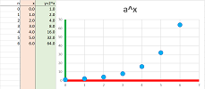
These are the possible values of $n$: $$... ,-3,-2,-1,0,1,2,3, ...$$ Note that we multiply by $2$ as we move right and divide by $2$ as we move left:

However, if we start at any point and proceed to the right, we only multiply. This means increase. A more general fact is true.

THEOREM (Monotonicity of Exponent). A geometric progression with ratio $a > 0$

• is increasing if $ a > 1$,
• is decreasing if $a < 1$.

This is what the graphs look like:

Exercise. Prove the theorem.

Exercise. If bacteria double in number every day and the current population is $1024$, how many were there two days ago?

The domain still misses some of the numbers that interest us! Suppose bacteria double in number every day starting with $1$. What happens after $10.5$ days? $$n=10.5, \quad 2^{10.5} = ?$$ We address fractional exponents in Chapter 4.

The Binomial Formula

We know that we aren't supposed to distribute powers over addition (an unforgivable mistake!): $$(a+b)^2\ne a^2+b^2.$$ To find what it is equal to we distribute multiplication over addition: $$\begin{array}{lll} (a+b)^2&=(a+b)\cdot (a+b)\\ &=(a+b)\cdot a +(a+b)\cdot b\\ &=(a\cdot a +b\cdot a)+(a\cdot b +b\cdot b)\\ &= a^2+2ab+b^2. \end{array}$$ The meaning of the formula is revealed if we interpret $(a+b)^2$ as the area of a square with side $a+b$:

The “end” terms are the two cubes and the “intermediate” terms are the rectangles.

The result is a handy formula: $$\begin{array}{|c|}\hline \quad (a+b)^2= a^2+2ab+b^2. \quad \\ \hline\end{array}$$ It is very useful, especially when we need to factor an expression; we simply read the formula from right to left: $$a^2+2ab+b^2=(a+b)^2.$$

Example (complete square). To factor $4x^2+4x+1$, we match it with the left-hand side of the formula above: $$\begin{array}{ll} &a^2&+&2ab&+&b^2&=&(a+b)^2\\ &4x^2&+&4x&+&1&=&?\\ \Longrightarrow&a^2=4x^2&&..&&b^2=1\\ \Longrightarrow&a=2x&&..&&b=1\\ \Longrightarrow&4x^2&+&4x&+&1&=&(2x+1)^2\\ \end{array}$$ The middle term also checks out. $\square$

Exercise. Factor $9x^2+12xy+4y^2$.

What about the higher powers? To get the cubic power (and beyond), we continue multiplying by $(a+b)$ and applying the Distributive Property: $$\begin{array}{lll} (a+b)^3&=(a+b)^2\cdot (a+b)\\ &=(a^2+2ab+b^2)\cdot (a+b)\\ &=(a^2+2ab+b^2)\cdot a +(a^2+2ab+b^2)\cdot b\\ &=(a^2\cdot a+2ab\cdot a+b^2\cdot a )+(a^2\cdot b+2ab\cdot b+b^2\cdot b)\\ &= (a^3+2a^2b+ab^2)+(a^2b+2ab^2+b^3)\\ &=a^3+3a^2b+3ab^2+b^3. \end{array}$$

The result is another handy formula: $$\begin{array}{|c|}\hline \quad (a+b)^3= a^3+3a^2b+3ab^2+b^3. \quad \\ \hline\end{array}$$

Example (complete cube). To factor $x^3+3x^2+3x+1$, we match it with the left-hand side of the formula above: $$\begin{array}{ll} &a^3&+&3a^2b&+&3ab^2&+&b^3&=&(a+b)^3\\ &x^3&+&3x^2&+&3x&+&1&=&?\\ \Longrightarrow&a^3=x^3&&..&..&&&b^3=1\\ \Longrightarrow&a=x&&..&..&&&b=1\\ \Longrightarrow&x^3&+&3x^2&+&3x&+&1&=&(x+1)^3\\ \end{array}$$ The “intermediate” terms also checks out. $\square$

Exercise. Interpret $(a+b)^3$ as the volume of a cube with side $a+b$ and illustrate the meaning of the “intermediate” terms in the above formula.

The two-term expression $a+b$ is called a binomial. In the formula, $$(a+b)^m=a^m+...+b^m,$$ we call the left-hand side a binomial power and the right-hand side the binomial expansion.

As we arrange the terms according to the decreasing powers of $a$, a pattern starts to emerge! As the power of $a$ is decreasing, that of $b$ is increasing. Moreover, the combined power of $a$ and $b$, i.e., the sum of the two powers of each term, is $m=3$, just as it was $m=2$ in the last formula. Let's make a table that starts with $m=1$: $$\begin{array}{l|ccccc} \hline m=1&(a+b)^1&=& a^1&+&b^1\\ \text{powers:}&1&=&1+0&=&0+1\\ \hline m=2&(a+b)^2&=& a^2&+&2a^1b^1&+&b^2\\ \text{powers:}&2&=&2+0&=&1+1&=&0+2\\ \hline m=3&(a+b)^3&=&a^3&+&3a^2b^1&+&3a^1b^2&+&b^3\\ \text{powers:}&3&=&3+0&=&2+1&=&1+2&=&0+3\\ \hline m=4&(a+b)^4&=&a^4&+&?a^3b^1&+&?a^2b^2&+&?a^1b^3&+&b^4\\ \text{powers:}&4&=&4+0&=&3+1&=&2+2&=&1+3&=&0+4\\ \hline \end{array}$$ We also included -- as a guess -- the case $m=4$. Below we put the results in the spreadsheet with the formula: $$\texttt{ =RC2+R2C }.$$ The expansions above follow the diagonal as marked:

In each, the combined power of $a$ and $b$ remains the same and it grows by $1$ as move to the next diagonal.

The behavior of the powers is clear; it's the coefficients that represent a challenge. Let's state the former first.

THEOREM. The expansion of the $m$th power $(a+b)^m$ of the binomial $(a+b)$ consists of $m+1$ terms each of which has the sum of powers of $a$ and $b$ equal to $m$.

Proof. If $(a+b)^m$ has all terms with the sum of powers equal to $m$, then what happens in $$(a+b)^{m+1}=(a+b)^m\cdot (a+b)?$$ According to the Distributive Property, each of these terms is multiplied by $a$ or by $b$. Therefore, the total power goes up by $1$! $\blacksquare$

Exercise. Provide the missing parts of the proof.

In the summary below the coefficients of the terms remain unknown: $$\begin{array}{l|ccccc} \hline m&(a+b)^m&=&a^m&+&?a^{m-1}b^1&+&?a^{m-2}b^2&+...+&?a^2b^{m-2}&+&?a^1b^{m-1}&+&b^m\\ \text{powers:}&m&=&m+0&=&(m-1)+1&=&(m-2)+2&=...=&2+(m-2)&=&1+(m-1)&=&0+m\\ \hline \end{array}$$ As you can see, the last row just shows all possible ways to represent $m$ as a sum of two non-negative integers. A pattern is partially visible: $$\begin{array}{l|ccccc} \hline m=1&(a+b)^1&=& a^1&+&b^1\\ \text{coefficients:}&&&1&&1\\ \hline m=2&(a+b)^2&=& a^2&+&2a^1b^1&+&b^2\\ \text{coefficients:}&&&1&&2&&1\\ \hline m=3&(a+b)^3&=&a^3&+&3a^2b^1&+&3a^1b^2&+&b^3\\ \text{coefficients:}&&&1&&3&&3&&1\\ \hline m=4&(a+b)^4&=&a^4&+&?a^3b^1&+&?a^2b^2&+&?a^1b^3&+&b^4\\ \text{coefficients:}&&&1&&4&&?&&4&&1\\ \hline \end{array}$$ We've made a guess in the last row but the middle term is still unknown.

An actual computation reveals that it's $6$: $$\begin{array}{l|ccccc} m=1&1&&1\\ m=2&1&&2&&1\\ m=3&1&&3&&3&&1\\ m=4&1&&4&&6&&4&&1\\ \end{array}$$ This is how things develop in this table: $$\begin{array}{l|ccccc} m=3&1&+&3&\\ &&&||&&\\ m=4&1&&4&&\\ \end{array}\quad\begin{array}{ccccc} 3&+&3&\\ &&||&&\\ 4&&6&&\\ \end{array}\quad\begin{array}{ccccc} 3&+&1&\\ &&||&&\\ 6&&4&&\\ \end{array}$$ Every two adjacent terms are added and placed in the next row.

The table is a sequence of sequences and the values in the next row are determined by the ones in the last. It is more convenient, however, to arrange the terms in an isosceles instead of a right triangle as above. This how we build $4$th row from the $3$rd: $$\begin{array}{l|ccccc} m=3& &&&1&&&&3&&&&3&&&&1\\ & &&\swarrow&&\searrow&_{1+3}&\swarrow&&\searrow&_{3+3}&\swarrow&&\searrow&_{3+1}&\swarrow&&\searrow\\ m=4& &1&&&&4&&&&6&&&&4&&&&1\\ \end{array}$$ Each entry is the sum of the two entries above it. The result is called the Pascal Triangle: $$\begin{array}{l|ccccc} m=0&&&&&&&1&\\ m=1&&&&&&1&&1\\ m=2&&&&&1&&2&&1\\ m=3&&&&1&&3&&3&&1\\ m=4&&&1&&4&&6&&4&&1\\ m=5&&1&&5&&10&&10&&5&&1\\ ...&.&&.&&.&&.&&.&&.&&.\\ \end{array}$$ The computation may continue indefinitely.

THEOREM (Binomial Theorem). If two consecutive terms of the expansion of $(a+b)^m$ are $$Xa^nb^{m-n}\ \text{ and }\ Ya^{n-1}b^{m-n+1},$$ then the expansion of $(a+b)^{m+1}$ contains $$(X+Y)a^{n}b^{m-n+1}.$$

Proof. $$\begin{array}{lll} (Xa^nb^{m-n}+Ya^{n-1}b^{m-n+1})(a+b)&=Xa^nb^{m-n}a+Ya^{n-1}b^{m-n+1}a+Xa^nb^{m-n}b+Ya^{n-1}b^{m-n+1}b\\ &=Xa^{n+1}b^{m-n}+Ya^{n}b^{m-n+1}+Xa^nb^{m-n+1}+Ya^{n-1}b^{m-n+2}\\ &=Xa^{n+1}b^{m-n}+(X+Y)a^{n}b^{m-n+1}+Ya^{n-1}b^{m-n+2}.\\ \end{array}$$ $\blacksquare$

Exercise. Provide the missing parts of the proof.

Example. This is how the Pascal Triangle is used. Let's take its $5$th row and produce a binomial expansion: $$\begin{array}{lllll} m=5&&1&&5&&10&&10&&5&&1\\ (a+b)^5=&&1\cdot a^5&+&5\cdot a^4b&+&10\cdot a^3b^2&+&10\cdot a^2b^3&+&5\cdot ab^4&+&1\cdot b^5\\ \end{array}$$ $\square$

One can easily compute, recursively, a large part of the Pascal triangle with a spreadsheet:

We use the formula: $$\texttt{=R[-1]C[-1]+R[-1]C[1]}.$$

So, for each $m$, we have a sequence of $m+1$ integers: $$\begin{array}{c|cc} n&0& 1& ... &m-1& m\\ \hline &1& m& ... &m& 1& \end{array}$$

Definition. The $n$th term of this sequence is called the binomial coefficient and is denoted by: $$\binom{m}{n}.$$

The Pascal Triangle takes the form: $$\begin{array}{ccccc} &&&&&&&\binom{0}{0}&\\ &&&&&&\binom{1}{0}&&\binom{1}{1}\\ &&&&&\binom{2}{0}&&\binom{2}{1}&&\binom{2}{2}\\ &&&&\binom{3}{0}&&\binom{3}{1}&&\binom{3}{2}&&\binom{3}{3}\\ &&&.&&.&&.&&.&&.&&\\ \end{array}$$ The first number indicates the row and the second the position within the row.

Exercise. Show that $$\binom{m}{n}=\binom{m}{m-n}.$$

Exercise. Show that $$\binom{m}{2}=m.$$

Then the Binomial Theorem is restated as follows.

Corollary. $$\binom{m}{n}+\binom{m}{n+1}=\binom{m+1}{n+1}.$$

This is the recursive formula. What is the $n$th term formula for this sequence or rather sequences?

THEOREM (Binomial Coefficient). For every positive integers $m$ and $n$, we have: $$\binom{m}{n} =\frac{m!}{n!(m-n)!}.$$

Proof. We confirm the recursive formula: $$\begin{array}{lll} \binom{m}{n}+\binom{m}{n+1}&=\frac{m!}{n!(m-n)!}+\frac{m!}{(n+1)!(m-n-1)!}\\ &=\frac{m!}{n!(m-n-1)!(m-n)}+\frac{m!}{n!(m-n-1)!(n+1)}\\ &=\frac{m!(n+1)+m!(m-n)}{n!(m-n-1)!(m-n)(n+1)}\\ &=\frac{m!\big( (n+1)+(m-n)\big)}{(n+1)!(m-(n+1))!}\\ &=\frac{m!\big( m+1\big)}{(n+1)!(m-(n+1))!}\\ &=\binom{m+1}{n+1}. \end{array}$$ $\blacksquare$

Warning: even though a fraction, a binomial coefficient is an integer.

Example. To confirm, we substitute $m=5$ and $n=3$: $$\binom{5}{3} =\frac{5!}{3!(5-3)!}=\frac{5!}{3!2!}=\frac{2\cdot 3\cdot 4 \cdot 5}{2\cdot 3\cdot 2}=2 \cdot 5=10.$$ The result matches the one in the Pascal Triangle. $\square$

The binomial coefficient can also be interpreted in combinatorial terms. Since $$(a+b)^m=\underbrace{(a+b)\cdot (a+b)\cdot ... \cdot (a+b)}_{m\text{ times}},$$ there will be one term in the binomial expansion for each choice of either $a$ or $b$ from each of the factors: $$a^nb^{m-n}=\underbrace{a\cdot a\cdot ... \cdot a}_{n\text{ times}}\cdot\underbrace{b\cdot b\cdot ... \cdot b}_{m-n\text{ times}}.$$

THEOREM. The binomial coefficient $\binom{m}{n}$ is the number of ways we can choose $n$ objects from $m$.

Example. In how many ways can one form a team of $5$ from $20$ players? We compute: $$\begin{array}{ll} \binom{20}{5} &=\frac{20!}{5!15!}\\ &=\frac{15!\cdot 16\cdot 17\cdot 18 \cdot 19 \cdot 20}{5!15!}\\ &=\frac{16\cdot 17\cdot 18 \cdot 19 \cdot 20}{2\cdot 3\cdot 4 \cdot 5}\\ &=\frac{16\cdot 17\cdot 18 \cdot 19 }{2\cdot 3}\\ &=16\cdot 17\cdot 3 \cdot 19\\ &=15,504. \end{array}$$ $\square$

Exercise. How many different hands of $5$ are there in a deck of $52$ cards?

The sequence of differences: velocity

Sequences are subject to algebraic operations: addition, subtraction, multiplication, and division. These operations produce new sequences. However, there are two operations that also produce new sequences that tell us a lot about the original sequence: sums and differences. We saw them in action in the first section as locations and velocities (when the time intervals are equal to the time unit) respectively:

If the sequence represents the location, the difference can also represents the displacement.

In this section we start on the path of development of an idea that culminates with the first main concept of calculus, the derivative (Chapter 7).

The differences represent the change of the sequence, from each of its terms to the next.

Example (lists). If a sequence is given by a list, we subtract the last term from the current one and record it at the bottom row: $$\begin{array}{rcccccccc} \text{sequence:}&2&&&&4&&&&7&&&&1&&&&-1&&...\\ && \searrow&&\swarrow&&\searrow&&\swarrow&&\searrow&&\swarrow&&\searrow&&\swarrow&&&...\\ \text{differences:}&&\qquad&4-2&&&&7-4&&&&1-7&&&&-1-1&&&&...\\ \text{}&&&||&&&&||&&&&||&&&&||&&&&...\\ \text{new sequence:}&&&2&&&&3&&&&-6&&&&-2&&&&...\\ \end{array}$$ We have a new list. $\square$

On the diagram of the sequence, we just count the number of steps we make, up and down:

These increments then make a new sequence.

Definition. For a sequence $a_n$, its sequence of differences, or simply the difference, is a new sequence, say $d_n$, defined for each $n$ by: $$d_n=a_{n+1}-a_n,$$ and denoted by: $$\Delta a_n=a_{n+1}-a_n.$$

Warning: the notation $\Delta$ applies to the whole sequence $a_n$ and $\Delta a$ is seen as the name of the new sequence; the notation for the difference is an abbreviation for: $(\Delta a)_n$.

Warning: if the original sequence starts with $n=q$, then the new sequence starts with $n=q+1$ but it could also be arranged to start with $n=q$ or any other index.

This is what the definition says: $$\begin{array}{rcccccccc} \text{sequence:}&a_1&&&&a_2&&&&a_3&&&&a_4&&&&a_5&&...\\ && \searrow&&\swarrow&&\searrow&&\swarrow&&\searrow&&\swarrow&&\searrow&&\swarrow&&&...\\ \text{differences:}&&\qquad&a_2-a_1&&&&a_3-a_2&&&&a_4-a_3&&&&a_5-a_4&&&&...\\ \text{}&&&||&&&&||&&&&||&&&&||&&&&...\\ \text{new sequence:}&&&d_1&&&&d_2&&&&d_3&&&&d_4&&&&...\\ \text{}&&&||&&&&||&&&&||&&&&||&&&&...\\ \text{notation:}&&&\Delta a_1&&&&\Delta a_2&&&&\Delta a_3&&&&\Delta a_4&&&&...\\ \end{array}$$

Now, a couple of specific sequences...

THEOREM (Arithmetic progression). The sequence of differences of an arithmetic progression with increment $m$ is a constant sequence with the value equal to $m$.

Proof. We simply compute from the definition: $$d_n=\Delta (a_0+mn)=a_{n+1}-a_n=(a_0+b(m+1))-(a_0+mn)=m.$$ $\blacksquare$

This is what it looks like, zoomed out:

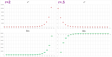
Let's take a look at the sequence of differences of a geometric progression with $a_0>0$. There are two cases:

We notice that the difference is positive and increasing when its ratio $r$ is larger than $1$ and it is negative and decreasing when $0<r<1$. It also resemble the original sequence.

THEOREM (Geometric progression). The sequence of differences of a geometric progression is a geometric progression with the same ratio.

Proof. If we have a geometric progression with ratio $r$ and initial term $a_0$, its formula is $a_n=a_0r^n$. Therefore, $$d_n=\Delta (a_0r^n)=a_{n+1}-a_n=a_0r^{n+1}-a_0r^n=a_0(r-1)\cdot r^n.$$ But this is a formula of a geometric progression with ratio $r$ and initial term $a_0(r-1)$. $\blacksquare$

Example (alternating sequence). The sequence of differences of the alternating sequence $a_n=(-1)^n$ is computed below: $$d_n=\Delta \left((-1)^n\right)=(-1)^{n+1}-(-1)^n=\begin{cases} (-1)-1,&n \text{ is even}\\ 1-(-1),&n\text{ is odd}\end{cases}=\begin{cases} -2,&n \text{ is even}\\ 2,&n\text{ is odd}\end{cases}=2(-1)^{n+1}.$$ $\square$

Exercise. What is the relation between the sequence above and its difference?

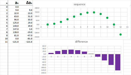
Example (motion). We can use computers to speed up these computations such as in the case when you have been recording your locations for a while. This is a spreadsheet formula of the sequence of differences (i.e., velocities): $$\texttt{=RC[-1]-R[-1]C[-1] }.$$ Whether the sequence comes from a formula or it's just a list of numbers, the above formula applies:

This is the result; a curve produces a new curve:

$\square$

Exercise. Describe what has happened referring to, separately, the first graph and the second graph.

Exercise. Imagine that the first column of the spreadsheet above is where you have been recording the monthly balance of your bank account. What does the second column represent? Describe what has been happening with your finances referring to, separately, the first graph and the second graph.

This is the time for some theory.

Consider this obvious statement about motion:

• “if I am standing still, my velocity is zero”.

The converse of this statement is as follows:

• “if my velocity is zero, I am standing still”.

If a sequence represents the position, we can restate this mathematically.

THEOREM (Constant). A sequence is constant if and only if its sequence of differences is zero; i.e., $$a_n\text{ is constant }\ \Longleftrightarrow\ \Delta a_n=0.$$

Proof. Direct: $$a_n=c\ \text{ for all }n\ \Longrightarrow\ a_{n+1}-a_n=c-c=0\ \Longrightarrow\ \Delta a_n=0.$$ Converse: $$a_{n+1}=a_n=c\ \text{ for all }n\ \Longleftarrow\ a_{n+1}-a_n=0\ \Longleftarrow\ \Delta a_n=0.$$ $\blacksquare$

Exercise. The difference of an arithmetic progression is constant and, conversely, if the difference of a sequence is constant sequence, the sequence is an arithmetic progression.

Consider this obvious statement about motion:

• “if I am moving forward, my velocity is positive”; and conversely,
• “if my velocity is positive, I am moving forward”.

We can restate this mathematically.

THEOREM (Monotonicity). A sequence is increasing/decreasing or constant, if and only if the sequence of differences is a positive/negative or zero; i.e., $$\begin{array}{ll} a_n&\text{ is increasing }&\ \Longleftrightarrow\ &\Delta a_n&\ge 0,\\ a_n&\text{ is decreasing }&\ \Longleftrightarrow\ &\Delta a_n&\le 0. \end{array}$$

Proof. $$a_{n+1}\ge a_n\ \text{ for all }n\ \Longleftrightarrow\ a_{n+1}-a_n\ge 0\ \Longleftrightarrow\ \Delta a_n\ge 0.$$ $\blacksquare$

Suppose now that there are two runners; we have a less obvious fact about motion:

• “if the distance between two runners isn't changing, then they run with the same velocity”, and vice versa,
• “if two runners run with the same velocity, the distance between them isn't changing”.

It's as if they are holding the two ends of a pole without pulling or pushing.

It is even possible that they speed up and slow down all the time. Once again, for sequences $a_n$ and $b_n$ representing their position, we can restate this idea mathematically in order to confirm that our theory makes sense.

Corollary. Two sequences differ by a constant if and only if their sequences of differences are equal; i.e., $$a_n-b_n\text{ is constant } \ \Longleftrightarrow\ \Delta a_n = \Delta b_n .$$

Proof. The corollary follows from the Constant Theorem above. $\blacksquare$

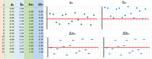
Example (spreadsheet). We shift the sequence $a_n$ below by $1$ unit up to produce a new sequence $b_n$ (top):

Because the ups and downs remain the same, the sequences of differences of these two sequences are identical (bottom). $\square$

Exercise. What of the two runners holding the pole also start to move their hands back and forth?

We can use the latter theorem to watch after the distance between the two runners. A matching statement about motion is:

• “if the distance from one of the two runners to the other is increasing, the former's velocity is higher”; and conversely,
• “if the velocity of one runner is higher than the other, the distance between them is increasing”.

We can restate this mathematically.

Corollary. The difference of two sequences is increasing or constant if and only if the former's difference is bigger than the latter's; i.e., $$\begin{array}{ll} a_n-b_n&\text{ is increasing }& \ \Longleftrightarrow\ &\Delta a_n& \ge &\Delta b_n,\\ a_n-b_n&\text{ is decreasing }& \ \Longleftrightarrow\ &\Delta a_n& \le &\Delta b_n . \end{array}$$

Proof. The corollary follows from the Monotonicity Theorem above. $\blacksquare$

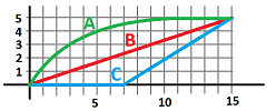
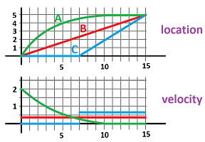
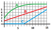
Example (runners). The graph shows the positions of three runners in terms of time, $n$. Describe what has happened.

They are all at the start line together and at the end they are all at the finish line. Furthermore, $A$ reaches the finish line first and $B$ and $C$ later who also starts late. This is how each did it:

• $A$ starts fast, then slows down, and almost stops close to the finish line;
• $B$ maintains the same speed;
• $C$ starts late and then runs fast at the same speed.

We can see that $A$ is running faster because the distance from $B$ is increasing. It becomes slower later which is visible from the decreasing distance. We can discover this and the rest of the facts by examining the graphs of the differences of the sequences:

$\square$

Exercise. Suppose a sequence is given by the graph for velocity above. Sketch the graph of the difference of this sequence. What is its meaning?

Exercise. Plot the location and the velocity for the following trip: “I drove fast, then gradually slowed down, stopped for a very short moment, gradually accelerated, hit a wall”. Make up your own story and repeat the task.

Exercise. Draw a curve on a piece of paper, imagine that it represents your locations, and then sketch what your velocity would look like. Repeat.

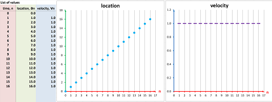
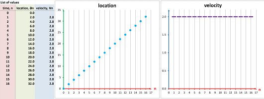
Example (driving). Driving forward at constant speed, i.e., we progress $2$ miles every minute:

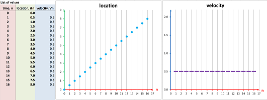
What if we drive slowly, covering only $1/2$ mile every minute?

This is, once again, a straight line but not as steep! Driving to the left at constant speed $2$ miles every minute:

Driving, stopping, and then resuming driving, backwards, at a higher speed:

The speed is constantly increasing:

$\square$

Exercise. Represent a round trip.

Example (paths). If we shrink these graphs horizontally, the time axis disappears. With only the location left, we then can imagine that we see a stroboscopic snapshot of motion (light it turned on for an instant at equal intervals):

It is called the path. We see in the former case that the distance covered during each interval is the same (constant speed) and in the latter case this distance is increasing (accelerated motion). $\square$

Example (difference quotient). How do we treat motion when the time increments aren't integers? What is the velocity then? Suppose $x_n$ and $y_n$ are two sequences. Then their difference quotient is defined to be the difference of $y_n$ over the difference of $x_n$: $$\frac{\Delta y_n}{\Delta x_n}=\frac{y_{n+1}-y_n}{x_{n+1}-x_n}.$$ It is the relative change -- the rate of change -- of the two sequences.

The difference quotient of the sequence of the location with respect to the sequence of time is the velocity. Finally, how do we treat motion when the time varies continuously instead of incrementally? What is the velocity then? This study resumes in Chapter 7. $\square$

The sequence of the sums: displacement

In the first section, we saw locations and velocities in action. We will look at the latter in this section:

In this section we start on the path of development of an idea that culminates with the second main concept of calculus, the integral (Chapter 11).

The sum represents the totality of the part of the sequence, found by adding each of its terms to the next, up to that point.

Example (lists). We add the current term to what we have accumulated so far: $$\begin{array}{cccc} \text{sequence:}&2&&4&&&&7&&&&1&&&&-1&&&...\\ &\downarrow&&\downarrow&&&&\downarrow&&&&\downarrow&&&&\downarrow&&&...\\ \text{sums:}&2&\\ &2&+&4&=&6\\ &&&&&6&+&7&=&13\\ &&&&&&&&&13&+&1&=&14\\ &&&&&&&&&&&&&14&+&(-1)&=&13\\ &\downarrow&&&&\downarrow&&&&\downarrow&&&&\downarrow&&&&\downarrow&...\\ \text{new sequence:}&2&&&& 6&&&& 13&&&& 14&&&& 13&...\\ \end{array}$$ We have a new list. $\square$

In the diagram of the sequence, we just stack up the bars one by one:

These stacked bars then make a new sequence.

In the beginning of the chapter, we learned how adding the progress of the car during each of the time period -- a sequence -- will give you the whole displacement. Once can see below how the terms of the original sequence are stacked up on top of each other, more and more:

In contrast to the difference, the sum must be defined (and possibly computed too) in a recursive manner.

Definition. For a sequence $a_n$, its sequence of sums, or simply the sum, is a new sequence $s_n$ defined and denoted for each $n\ge m$ within the domain of $a_n$ by a recursive formula: $$s_m=0,\quad s_{n+1}=s_n+a_{n+1};$$ denoted by: $$s_n=a_{m}+a_{m+1}+...+a_n,$$ or $$s_n=\sum_{k=m}^n a_k.$$

Example (alternating). Let's do some algebra. Here $a_n$ is the original sequence and $s_n$ is the new one: $$\begin{array}{c|c|lll} n&a_n&s_n&=&s_n\\ \hline 1&1&1&=&1\\ 2&-1&1-1&=&0\\ 3&1&1-1+1&=&1\\ \vdots&\vdots&\vdots&&\vdots\\ n&(-1)^n&1-1+1-...+(-1)^n&=&1\text{ or }0\\ \end{array}$$ $\square$

Let's take a closer look at the new notation. The first choice of how to represent the sum of a segment -- from $m$ to $n$ -- of a sequence $a_n$ is this: $$\underbrace{a_{m}}_{\text{step } 1}\quad \underbrace{+a_{m+1}}_{\text{step } 2}\ + ... \quad\underbrace{+a_{k}}_{\text{step } k}\ + ... \quad \underbrace{+a_{n}}_{\text{step }n-m}. $$ This notation reflects the recursive nature of the process but can also be repetitive and cumbersome. The second choice is more compact: $$\sum_{k=m}^{n}a_k.$$ Here the Greek letter $\Sigma$ stands for the letter S meaning “sum”. This is called the sigma notation.

Example. This is how the sigma notation is deconstructed: $$\sum_{k=0}^3 \big(k^2 + k \big) =20\qquad\leadsto\qquad\begin{array}{rlrll} \text{beginning}&\text{and end values for }k\\ \downarrow&\\ \begin{array}{r}3\\ \\k=0\end{array}&\sum \big(\quad k^2 + k \quad\big) &=&20.\\ &\qquad\qquad\uparrow&&\uparrow\\ &\qquad\text{a specific sequence}&&\text{a specific number} \end{array}$$ The computation above is expanded here: $$\sum_{k=0}^3 \big(k^2 + k \big)=\begin{array}{l|ll} k&k^2 + k\\ \hline 0&0^2 + 0&=0&_+\\ 1&1^2 + 1&=2&_+\\ 2&2^2 + 2&=6&_+\\ 3&3^2 + 3&=12&\\ \hline &&=20 \end{array}$$ $\square$

Exercise. Hoe will the sum change if we replace $k=0$ with $k=1$, or $k=-1$? What if we replace $3$ at the top with $4$?

Example. This is how we contract the summation: $$1^2 + 2^2 + 3^2 + ... + 17^2 = \sum_{k=1}^{n} k^2.$$ It is only possible if we find the $n$th term formula for the sequence: $a_k=k$. And this is how we expand back from this compact notation, by plugging the values of $k=1,2, ...,17$ into the formula: $$\sum_{k=1}^{17} k^2 = \underbrace{1^2}_{k=1} + \underbrace{2^2}_{k=2} + \underbrace{3^2}_{k=3} + ... + \underbrace{17^2}_{k=17}.$$ Similarly, $$1+\frac{1}{2}+\frac{1}{4}+\frac{1}{8}+...+\frac{1}{32}=\sum_{k=0}^{5} \frac{1}{2^k}.$$ $\square$

Exercise. Confirm that we can start at any other initial index if we just modify the formula: $$1+\frac{1}{2}+\frac{1}{4}+\frac{1}{8}+...+\frac{1}{32}=\sum_{k=1}^{6} \frac{1}{2^{k-1}}=\sum_{k=2}^{7} \frac{1}{2^{k-2}}=...$$

Exercise. Contract this summation: $$1+\frac{1}{3}+\frac{1}{9}+\frac{1}{27}=?$$

Exercise. Expand this summation: $$\sum_{k=0}^{4} (k/2)=?$$

Exercise. Rewrite using the sigma notation:

• (a) $1+3+ 5+ 7+ 9+ 11+ 13+ 15$;
• (b) $.9+ .99+ .999+ .9999$;
• (c) $1/2 -1/4+ 1/8 -1/16$;
• (d) $1+ 1/2+ 1/3+ 1/4+ ...+ 1/n$;
• (e) $1+1/2+1/4+1/8$;
• (f) $2+ 3+ 5+ 7+ 11+ 13+ 17$;
• (g) $1 -4+ 9 -16+ 25$.

Example (binomials). In this notation, the Binomial Theorem reads: $$(a+b)^m=\sum_{n=0}^m\binom{m}{n}a^{m-n}b^n.$$ For example, $$\begin{array}{rrrr} (a+b)^4&=&\sum_{n=0}^4\binom{4}{n}a^{4-n}b^n\\ &=&\binom{4}{0}a^{4-0}b^0&+&\binom{4}{1}a^{4-1}b^1&+&\binom{4}{2}a^{4-2}b^2&+&\binom{4}{3}a^{4-3}b^3&+&\binom{4}{4}a^{4-4}b^4\\ &=&1\cdot a^{4}b^0&+&4\cdot a^{3}b^1&+&6\cdot a^{2}b^2&+&4\cdot a^{1}b^3&+&1\cdot a^{0}b^4\\ &=&a^{4}&+&4 a^{3}b&+&6 a^{2}b^2&+&4ab^3&+&b^4\\ \end{array}$$ $\square$

The notation applies to all sequences, both finite and infinite. For infinite sequences, indicated by “...” at the end, the sum sequence is also called the series to be discussed in Chapter 15 ($s_n$ is then called the partial sum).

This is the definition of the sequence of sums written with the sigma notation: $$\begin{array}{cccc} \text{sequence:}&a_1&&a_2&&&&a_3&&&&a_4&&&&a_5&&&...\\ &\downarrow&&\downarrow&&&&\downarrow&&&&\downarrow&&&&\downarrow&&&...\\ \text{sums:}&a_1&\\ &a_1&+&a_2&=&s_2\\ &&&&&s_2&+&a_3&=&s_3\\ &&&&&&&&&s_3&+&a_4&=&s_4\\ &&&&&&&&&&&&&s_4&+&a_5&=&s_5\\ &\downarrow&&&&\downarrow&&&&\downarrow&&&&\downarrow&&&&\downarrow&...\\ \text{sequence of sums:}&s_1&&&& s_2&&&& s_3&&&& s_4&&&& s_5&...\\ &||&&&& ||&&&& ||&&&& ||&&&& ||&...\\ \text{sigma notation:}&\sum_{k=1}^{1}a_k&&&& \sum_{k=1}^{2}a_k&&&& \sum_{k=1}^{3}a_k&&&& \sum_{k=1}^{4}a_k&&&& \sum_{k=1}^{5}a_k&...\\ \end{array}$$

THEOREM (Arithmetic progression). The sum of an arithmetic progression with increment $m$ and a $0$ initial term is a (quadratic) sequence given by: $$\sum_{k=1}^{n} (mk) =\frac{n(n+1)}{2}m.$$

Exercise. Prove the theorem. Hint: use the example about round robins.

Example (series). What does the sum $$\frac{1}{2}+\frac{1}{4}+\frac{1}{8}+...$$ compute? We can see these terms as the areas of the squares below:

On the one hand, adding the areas of these squares will never go over $1$, the area of the big square, and, on the other, these squares seem to exhaust it... So, even the infinite sum sometimes makes sense (to be considered in Chapter 15). $\square$

We can notice that a certain pattern about the sum of a geometric progression:

Its sequence of sums resembles it...

THEOREM (Geometric progression). The sum of a geometric progression with ratio $\ne 1$ is a geometric progression with the same ratio plus a constant.

Proof. Below, we use a clever trick to get rid of “...”. We write the $n$th sum $s_n$, $$\begin{array}{lllll} s_n &=ar^0 &+ ar^1 &+ ar^2 &+ ... &+ ar^{n-1} &+ ar^n, \end{array}$$ and then multiply it by $r$: $$\begin{array}{lllll} rs_n&=r\big( ar^0 &+ ar^1 &+ ar^2 &+ ... &+ ar^{n-1} &+ ar^n \big)\\ &=\quad ar^1 &+\quad ar^2 &+\quad ar^3 &+ ... &+\quad ar^{n} &+\quad ar^{n+1}. \end{array}$$ Now we subtract these two: $$\begin{array}{lllll} s_n &=ar^0 &+ ar^1 &+ ar^2 &+ ... &+ ar^{n-1} &+ ar^n&\\ \quad rs_n&=\quad ar^1 &+\quad ar^2 &+\quad ar^3 &+ ... &+\quad ar^{n} &+\quad ar^{n+1}\\ \hline s_n-rs_n&=ar^0-ar^1 &+ ar^1-ar^2 &+ ar^2-ar^3 &+ ... &+ ar^{n-1}-ar^{n}&+ar^n-ar^{n+1}\\ &=ar^0 & & & &&\quad\qquad -ar^{n+1}. \end{array}$$ We cancel the terms that appear twice in the last row and “...” is gone! Therefore, $$s_n(1-r)=a-ar^{n+1}.$$ Thus, we have an explicit formula for the $n$th term of the sum: $$s_n=\frac{a}{1-r}(1-r^{n+1})=-\frac{a}{1-r}\cdot r^{n+1}+\frac{a}{1-r}.$$ The former is the geometric part and the latter is constant. $\blacksquare$

Exercise. Find the explicit formula for the sequence of sums of the alternating sequence $a_n=(-1)^n$.

Warning: the ability to produce explicit formulas for the $n$th terms of the sum is an exception not a rule.

Example (motion). We can use computers to speed up these computations such as in the case when you have been recording your velocities for a while. This is a formula for a spreadsheet (the locations): $$\texttt{=R[-1]C+RC[-1] }.$$ Whether the sequence comes from a formula or it's just a list of numbers, the above formula applies:

This is the result; a curve produces a new curve:

$\square$

Exercise. Describe what has happened referring to, separately, the first graph and the second graph.

Exercise. Imagine that the first column of the spreadsheet is where you have been recording your monthly deposit/withdrawals at your bank account. What does the second column represent? Describe what has been happening referring to, separately, the first graph and the second graph.

This is the time for some theory.

Recall this pair of obvious statements about motion:

• “if I am standing still, my velocity is zero”, and, vice versa,
• “if my velocity is zero, I am standing still”.

If the velocity is represented by a sequence, we can restate this mathematically using the sums.

THEOREM (Constant). The sequence of sums of a sequence is constant if and only if the sequence has only zero values starting from some term $N$; i.e., $$\sum_{k=m}^{n} a_k\text{ is constant }\ \Longleftrightarrow\ a_n=0\ \text{ for all }n\ge N.$$

Proof. $$\sum_{k=m}^{n} a_k=c\ \text{ for all }n\ \Longleftrightarrow\ a_{n+1}=\sum_{k=m}^{n+1} a_k -\sum_{k=m}^{n} a_k=c-c=0\ \Longleftrightarrow\ a_{n+1}=0.$$ $\blacksquare$

Here is another pair of statements about motion:

• “if I am moving forward, my velocity is positive”, and, vice versa,
• “if my velocity is positive, I am moving forward”.

We can restate this mathematically using the sums.

THEOREM (Monotonicity). The sequence of sums of a sequence is increasing if and only if the terms of the sequence are non-negative; i.e., $$\begin{array}{ll} \sum_{k=m}^{n} a_k&\text{ is increasing }&\ \Longleftrightarrow\ &a_n&\ge 0,\\ \sum_{k=m}^{n} a_k&\text{ is decreasing }&\ \Longleftrightarrow\ &a_n&\le 0. \end{array}$$

Proof. $$\sum_{k=m}^{n+1} a_k \ge \sum_{k=m}^{n} a_k\ \text{ for all }n\ \Longleftrightarrow\ a_{n+1}=\sum_{k=m}^{n+1} a_k -\sum_{k=m}^{n} a_k\ge 0.$$ $\blacksquare$

Now there are two runners:

• “if the distance between two runners isn't changing, then they run with the same velocity”, and, vice versa,
• “if two runners run with the same velocity, the distance between them isn't changing”.

Corollary. The sequences of sums of two sequences differ by a constant if and only if the sequences are equal starting with some term $N$; i.e., $$\sum_{k=m}^{n} a_k-\sum_{k=m}^{n} b_k\text{ is constant } \ \Longleftrightarrow\ a_n = b_n \ \text{ for all }n\ge N.$$

Proof. The corollary follows from the Constant Theorem above. $\blacksquare$

Example. We have two different sequences $a_n$ and $b_n$ that become identical after $3$ terms.

The result is that the sum of the latter sequence is just a vertical shift of the sum of the former:

To state this algebraically, for all $n$ we have: $$\sum_{k=m}^{n} a_k=\sum_{k=m}^{n} b_k +C,$$ where $C$ is some number. Similarly, we have two identical sequences $a_n$ and $b_n$ but the computation of their sequences of sums starts at different points:

$\square$

Exercise. What is the meaning of the number $C$?

We can use the latter theorem to watch after the distance between the two runners. A matching statement about motion is:

• “if the distance from one of the two runners to the other is increasing, the former's velocity is higher”, and, vice versa,
• “if the velocity of one runner is higher than the other, the distance between them is increasing”.

We can restate this mathematically using the sums.

Corollary. The difference of the sequences of sums of two sequences is increasing if and only if the corresponding terms of the former is larger than or equal to those of the latter; i.e., $$\begin{array}{ll} \sum_{k=m}^{n} a_k-\sum_{k=m}^{n} b_k&\text{ is increasing }& \ \Longleftrightarrow\ &a_n& \ge &b_n,\\ \sum_{k=m}^{n} a_k-\sum_{k=m}^{n} b_k&\text{ is decreasing }& \ \Longleftrightarrow\ &a_n& \le &b_n. \end{array}$$

Proof. The corollary follows from the Monotonicity Theorem above. $\blacksquare$

Here is another way to look at the statement the faster covers the longer distance. It is about comparing the values of two sums. Consider this simple algebra: $$\begin{array}{lll} u&\le&U,\\ v&\le&V,\\ \hline u+v&\le&U+V.\\ \end{array}$$ The rule applies even if we have more than just two terms: $$\begin{array}{rcl} u_m&\le&U_m,\\ u_{m+1}&\le&U_{m+1},\\ \vdots&\vdots&\vdots\\ u_q&\le&U_q,\\ \hline u_m+...+u_q&\le&U_m+...+U_q. \end{array}$$

Example (runners). The graph shows the velocities of three runners in terms of time, $n$. Describe what has happened.

It's easy to describe how they are moving:

• $A$ starts fast and the slows down;
• $B$ maintains the same speed;
• $C$ starts late and then runs fast.

But where are they? These are several possible answers:

Which one is the right one depends on the starting point. $\square$

Exercise. Does what happened below match the description above?

Exercise. Suppose a sequence is given by the graph for location above. Sketch the graph of the sum of this sequence.

Exercise. Plot the location and the velocity for the following trip: “I drove slow, then gradually speeded up, stopped for a very short moment and started in the opposite direction, quickly accelerated and from that point maintained the speed”. Make up your own story and repeat the task.

Exercise. Draw a curve on a piece of paper, imagine that it represents your velocity, and then sketch what your locations would look like. Repeat.

Here is another trivial statement about motion: $$\begin{array}{lll} &\text{distance covered during the 1st hour }\\ +&\text{distance covered during the 2nd hour }\\ =&\text{distance during the two hours}. \end{array}$$ The statement is about the fact that, while adding, we can change the order of terms freely; this is called the Associativity Property of addition. At its simplest, it allows us to remove the parentheses: $$\begin{array}{rlcr} &(u_m+u_{m+1}+...+u_{q-1}+u_q)&+&(u_{q+1}+u_{q+2}+...+u_{r-1}+u_r)\\ =&u_m+u_{m+1}+...+u_{q-1}+u_q&+&u_{q+1}+u_{q+2}+...+u_{r-1}+u_r\\ =&u_m+u_{m+1}+&...&+u_{r-1}+u_r. \end{array}$$

An abbreviated version of this identity is as follows.

THEOREM (Additivity). The sum of the sums of two consecutive segments of a sequence is the sum of the combined segment; i.e., for any sequence $u_n$ and for any $m,q,r$ with $m\le q\le r$, we have: $$\sum_{k=m}^q u_k +\sum_{k=q+1}^r u_k = \sum_{k=m}^r u_k .$$

In addition to motion, sums are used for a certain task of data analysis -- averaging.

Definition. The mean (or the average) of a quantity given by $n$ numbers $a_1,...,a_n$ is defined to be: $$\text{mean }=\frac{a_1+a_2+...+a_n}{n}.$$

For example, this is the mean of a few random numbers:

If we start with a sequence $a_n$, a commonly considered new sequence is the average of $a_n$ over all of its segments of a given length, say $m$, as follows: $$b_n=\frac{a_{n-m}+a_n-m+1}+...+a_n}{m}=\frac{1}{m}\sum_{k=n-m}^n a_k.$$ It is called the running average. The example below ($m=5$) shows the running average “smooths out” the roughness of the sequence:

It is computed with the formulas: $$\texttt{ =sum(R[-4]C[-1]:RC[-1])/5}\ \text{ or }\ \texttt{ =AVERAGE(R[-4]C[-1]:RC[-1])}.$$

Exercise. Show that the running average of an increasing sequence is increasing.

Exercise. Give an example that shows that the running average delays exhibiting a change from increasing to decreasing behavior.

This study continues in Chapter 14.

Example (Riemann sums). Now do we treat motion when the time moments aren't integers? What is the displacement then? Suppose $x_n$ and $v_n$ are two sequences. Then their Riemann sum is defined to be the sequence of sums of the sequence of the product of $v_n$ and the difference of $x_n$: $$\sum_{k=1}^n v_n\, \Delta x_n.$$

We know from the last section that if $y_n$ is the position, then the velocity is $v_n=\Delta y_n/ \Delta x_n$. Therefore, the Riemann sum of the sequence of the velocity with respect to the sequence of time is the displacement. Finally, how do we treat motion when the time varies continuously instead of incrementally? What is the displacement then? This study resumes in Chapter 11. $\square$

Sums of differences and differences of sums: motion

In this section we start on the path of development of an idea that culminates with the cornerstone result of calculus, the Fundamental Theorem of Calculus (Chapter 11).

We know that addition and subtraction undo each other; it makes sense then that making the sequences of differences and making the sequences of sums will cancel each other in a similar manner!

Example (driving). We know how to get velocity from the location -- and the location from the velocity. We expect that executing these two operations consecutively should bring us back where we started.

Let's take another look at the example of two computations about motion -- a broken odometer and a broken speedometer -- presented in the beginning of this chapter. The terminology has now been developed: every time we speak of a sequence, its difference (also a sequence), and its sum (also a sequence).

In the first diagram, we first use the velocity to acquire the displacement via sums; but the differences of the latter are the former:

We are back to the original.

In the second diagram, we first use the location to acquire the velocity via differences; but the sums of the latter are the former:

We are back to the original (if we start at the same initial location). $\square$

Example (lists). Below we have a sequence given by a list. We compute its sequence sums and then compute the sequence of differences of the result: $$\begin{array}{cccc} \text{sequence:}&3&&1&&&&0&&&&-2&&&&1&&&...\\ &\downarrow&&\downarrow&&&&\downarrow&&&&\downarrow&&&&\downarrow&&&...\\ \text{sums:}&3&\\ &3&+&1&=&4\\ &&&&&4&+&0&=&4\\ &&&&&&&&&4&+&(-2)&=&2\\ &&&&&&&&&&&&&2&+&1&=&3\\ &\downarrow&&&&\downarrow&&&&\downarrow&&&&\downarrow&&&&\downarrow&...\\ \text{sequence of sums:}&3&&&& 4&&&& 4&&&& 2&&&& 3&...\\ && \searrow&&\swarrow&&\searrow&&\swarrow&&\searrow&&\swarrow&&\searrow&&\swarrow&&...\\ \text{differences:}&&\qquad&4-3&&&&4-4&&&&2-4&&&&3-2&&&...\\ \text{}&&&||&&&&||&&&&||&&&&||&&&...\\ \text{new sequence:}&&&1&&&&0&&&&-2&&&&1&&&...\\ \end{array}$$ We are back to the original sequence! $\square$

Exercise. What happened to the very first term?

Exercise. Start with the same sequence and use the diagrams to show that the sums of the differences give us the original sequence.

Now the general case.

Just comparing the illustrations above demonstrates that the two operations -- the difference and the sum -- undo the effect of each other:

As you can see in the picture, the sum (left to right) stacks up the terms of the sequence on top of each other while the difference (right to left) takes these apart.

Let's take care of the algebra. This is what we know.

(1) Suppose we have a sequence, $a_n$. We compute its difference, a new sequence: $$b_{n+1}=a_{n+1}-a_{n}.$$ (2) Suppose we have a sequence, $c_k$. We compute its sum, a new sequence: $$d_n=\sum_{k=1}^n c_k,$$ or, recursively: $$d_{n+1}=d_n+c_{n+1}.$$

We use this setup to answer the following two questions.

The first question we would like to answer is, what is the difference of the sum? We start with $c_n$. Then, we have from (2) and (1) respectively: $$d_{n+1}=d_n+c_{n+1} \ \text{ and }\ b_{n+1}=d_{n+1}-d_{n}.$$ We substitute the first formula into the second (and cancel): $$b_{n+1}=d_{n+1}-d_{n}=(d_n+c_{n+1})-d_n=c_{n+1}.$$ So, the answer is, the original sequence.

The second question we would like to answer is, what is the sum of the difference? We start with $a_n$. Then, we have from (1) and (2) respectively: $$b_{k}=a_{k}-a_{k-1} \ \text{ and }\ d_n=\sum_{k=1}^n b_k.$$ We substitute the first formula into the second (and cancel): $$d_n=\sum_{k=1}^n b_k=\sum_{k=1}^n (a_{k}-a_{k-1})=(a_{2}-a_{1})+(a_{3}-a_{2})+...+(a_{n}-a_{n-1})=-a_1+a_{n}.$$ So, the answer is, the original sequence plus a constant.

We summarize these results in the form of the following two theorems.

THEOREM (Fundamental Relation I). The difference of the sum of $a_n$ is $a_n$; i.e., for all $n$, we have: $$\Delta \bigg(\sum_{k=1}^n a_k \bigg)=a_n.$$

The two operations cancel each other!

THEOREM (Fundamental Relation II). The sum of the difference of $b_n$ is $b_n+C$, where $C$ is a constant; i.e., for all $n$, we have: $$\sum_{k=1}^n\left( \Delta b_k \right) =b_n+C.$$

The two operations -- almost -- cancel each other, again!

Example (spreadsheet). For larger sets of data, we use a spreadsheet. Recall the formulas.

• From a sequence to its sum:

$$\texttt{ =R[-1]C+RC[-1]}\ ,$$ and

• from a sequence to its difference:

$$\texttt{ =RC[-1]-R[-1]C[-1]}\ .$$ What if we combine the two consecutively? From a sequence to its difference to the sum of the latter:

It's the same curve! Now in the opposite order, from a sequence to its sum to the difference of the latter:

It's the same curve! $\square$

Example (falling ball). In an example from earlier in this chapter, we have experimental data of the heights of a ping-pong ball falling down:

Just as before, we use a spreadsheet to plot the location sequence, $p_n$ (green). We then compute the difference of $p_n$, i.e., the velocity, $v_n$ (purple):

It looks like a straight line! This take we take one more step -- we now compute the difference of the velocity sequence. It is the acceleration, $a_n$ (blue). It appears constant! $\square$

Example (shooting). If we accept the premise, developed in the last example, that the acceleration of free fall is constant, we can try to predict the behavior of an object shot in the air -- with any height and any initial velocity. The direction of our computation is opposite to that of the last example: we assume that we know the acceleration, then derive the velocity, and then derive the location (altitude) of the object in time. We use the sums:

Above, a projectile is launched from a $100$ meter tall building vertically up in the air with speed $100$ meters per second (the gravity causes acceleration of $-9.8$ meters per second squared). We can see that it will reach its highest point in about $20$ seconds and will hit the ground in about $40$ seconds. $\square$

Exercise. How high does the projectile go in the above example?

Exercise. Use the above example, how long will it take for the projectile to reach the ground if fired down?

Exercise. Use the above model to determine how long it will take for an object to reach the ground if it is dropped. Ask your own question about the situation and answer it. Repeat.

Exercise. Suppose the time is given by another sequence (an arithmetic progression). Compute the velocity and the acceleration from the table below: $$\begin{array}{r|ll} &\text{time}&\text{height}\\ n&t_n&a_n\\ \hline 1&.00&36\\ 2&.05&35\\ 3&.10&32\\ 4&.15&25\\ 5&.20&20\\ 6&.25&11\\ 7&.30&0 \end{array}$$

This study of motion continues throughout the book.

The algebra of sums and differences

What happens to the differences and the sums under algebraic operations on the sequences involved? There are a few shortcut properties.

Here is an elementary statement about motion:

• if two runners are running away from a post, their relative velocity is the sum of their respective velocities.

The idea of addition of the changes, i.e., the differences, is illustrated below:

Here, the bars that represent the change of the values of the sequence are stacked on top of each other, then the heights are added to each other and so are the height differences. The algebra behind this geometry is very simple: $$(A+B)-(a+b)=(A-a)+(B-b).$$ It's the Associative Rule of addition.

THEOREM (Sum Rule for differences). The difference of the sum of two sequences is the sum of their differences; i.e., for any two sequences $a_n,b_n$, their differences satisfy: $$\Delta(a_n+b_n)=\Delta a_n+\Delta b_n.$$

Proof. $$\begin{array}{lll} \Delta (a_n + b_n)&=(a_{n+1} + b_{n+1})- (a_n + b_n)\\ &=(a_{n+1}-a_{n})+ (b_{n+1} - b_n)&\\ &=\Delta a_n+\Delta b_n. \end{array}$$ $\blacksquare$

Example. Let's consider the sum of an arithmetic and a geometric progressions: $$\Delta (a+mn+ar^n)=\Delta (a+mn)+\Delta (ar^n)=m+ar^n(r-1).$$ $\square$

So, the theorem rephrases -- in terms of differences -- the idea that if two runners are running away from a post, their velocities are added in order to find the distance between them. But differences and sums are matched up according to the Fundamental Relations presented in the last section! It should be no surprise then that there is a matching theorem about sums.

When two sequences are added to each other, what happens to their sums? This simple algebra, the Associative Property combined with the Commutative Property, tells the whole story: $$\begin{array}{lll} &u&+&U,\\ +\\ &v&+&V,\\ \hline =&(u+v)&+&(U+V).\\ \end{array}$$ The rule applies even if we have more than just two terms; it's about re-arranging terms: $$\begin{array}{rcl|lll} u_p&+&U_p&(u_{p}+U_{p})+\\ u_{p+1}&+&U_{p+1}&(u_{p+1}+U_{p+1})+\\ \vdots&\vdots&\vdots&\quad\vdots\\ u_q&+&U_q&(u_q+U_q)\\ \hline =(u_p+...+u_q)&+&(U_p+...+U_q)&=(u_p+U_p)+&...&+(u_q+U_q). \end{array}$$

An abbreviated version of this formula is as follows.

THEOREM (Sum Rule for sums). The sum of the sums of two sequences is the sum of the sequence of sums; i.e., if $u_n$ and $U_n$ are sequences, then for any $p,q$ with $p\le q$, we have: $$\sum_{n=p}^{q} u_n+\sum_{n=p}^{q}U_n=\sum_{n=p}^{q} (u_n +U_n).$$

Exercise. Derive this theorem from the last one, reverse.

Here is another simple statement about motion:

• if the distance is re-scaled, such as from miles to kilometers, then so is the velocity -- at the same proportion.

The idea of proportional change is illustrated below:

Here, if the heights triple then so do the height differences. The algebra behind this geometry is very simple: $$kA-ka=k(A-a).$$ It's the Distributive Rule.

THEOREM (Constant Multiple Rule for differences). The difference of a multiple of a sequence is the multiple of the sequence's difference; i.e., for any sequence $a_n$, the differences satisfy: $$\Delta(ka_n)=k\Delta a_n.$$

Proof. $$\begin{array}{lll} \Delta (ka_n )&=ka_{n+1} k- ka_n\\ &=ka_{n+1} k- ka_n\\ &=k\Delta a_n. \end{array}$$ $\blacksquare$

The theorem can also be interpreted as follows: if the distances are proportionally increased, then so are the velocities needed to cover them, in the same period of time.

Is there a matching statement about sums? Yes, but let's first look at motion again: if your velocity is tripled, then so is the distance you have covered.

When a sequence is multiplied by a constant, what happens to its sums? This simple algebra, the Distributive Property, tells the whole story: $$\begin{array}{lll} c\cdot(&u&+&U)\\ =&cu&+&cU.\\ \end{array}$$ The rule applies even if we have more than just two terms; it's about factoring: $$\begin{array}{rcl|lll} c&\cdot&u_p&c\cdot u_p+\\ c&\cdot&u_{p+1}&c\cdot u_{p+1}+\\ \vdots&\vdots&\vdots&\quad\vdots\\ c&\cdot&u_q&c\cdot u_q\\ \hline =c\cdot u_p+&...&+c\cdot u_q&=c\cdot(u_p+...+u_q). \end{array}$$

An abbreviated version of this formula is as follows.

THEOREM (Constant Multiple Rule for sums). The sum of a multiple of a sequence is the multiple of its sum; i.e., if $u_n$ is a sequence, then for any $p,q$ with $p\le q$ and any real $c$, we have: $$ \sum_{n=p}^{q} (cu_n) = c\sum_{n=p}^{q} u_n .$$

Exercise. Derive this theorem from the last one, reverse.

Now we go beyond addition and multiplication by a constant.

Let's imagine this:

• if two runners are unfurling a flag (or a tarp) while running east and north respectively, what is happening to the area of this rectangle?

So, the products of two sequences are interpreted products as areas of the rectangles formed by the sequences, illustrated below:

As the width and the depth are increasing, so is the area of the rectangle. We can see that the increase of the area cannot be expressed entirely in terms of the increases of the width and depth! This increase is split into two parts corresponding to the two terms in the right-hand side of the formula below.

THEOREM (Product Rule for differences). The difference of the product of two sequences is found as a combination of these sequences and either of the two differences; for any two sequences $a_n,b_n$ the differences satisfy: $$\Delta (a_n \cdot b_n)=a_{n+1} \cdot \Delta b_n + \Delta a_n \cdot b_n.$$

Proof. $$\begin{array}{lll} \Delta (a_n \cdot b_n)&=a_{n+1} \cdot b_{n+1}- a_n \cdot b_n&\text{ ... insert terms in the middle...}\\ &=a_{n+1} \cdot b_{n+1}-a_{n+1} \cdot b_{n}+ a_{n+1} \cdot b_n- a_n \cdot b_n&\text{ ... factor...}\\ &=a_{n+1} \cdot (b_{n+1})-b_{n})+ (a_{n+1} - a_n) \cdot b_n&\text{}\\ &=a_{n+1} \cdot \Delta b+ \Delta a_n \cdot b_n. \end{array}$$ $\blacksquare$

Example. Let's consider the product of an arithmetic and a geometric progressions: $$\Delta (mn \cdot ar^n)=\Delta (mn)\cdot ar^n +mn\Delta(ar^n)=mar^n+mnar^n(r-1).$$ $\square$

Example (squares). The difference of the square sequence $a_n=n^2$ is computed with the Product Rule: $$\Delta (n^2)=\Delta (n\cdot n)=(n+1) \cdot \Delta (n) + \Delta (n) \cdot (n)=(n+1)+(n)=2n+1.$$ It's an arithmetic progression.

$\square$

Exercise. Find a formula for the difference of the power sequence, $\Delta n^m$, using the Binomial Theorem.

Example (reciprocals). Let's find the formula for the difference of the reciprocals: $$\Delta\left(\frac{1}{n}\right)=\frac{1}{n+1}-\frac{1}{n}=\frac{n-(n+1)}{n(n+1)}=-\frac{1}{n(n+1)}.$$ The sequence decreases but slower and slower.

$\square$

THEOREM (Quotient Rule for differences). The difference of the quotient of two sequences is found as a combination of these sequences and either of the two differences; for any two sequences $a_n,b_n$, the differences satisfy: $$\Delta \left(\frac{a_n}{b_n}\right)=\frac{a_{n+1} \cdot \Delta b_n + \Delta a_n \cdot b_n}{b_nb_{n+1}}.$$

Exercise. Prove the theorem.

There are no matching statements for sums as simple as these two.