Precalculus

The coordinate system for dimension $1$

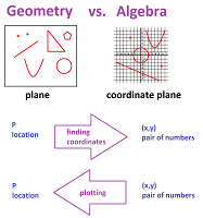
The idea of a coordinate system is to transition from

• geometry: points, then lines, triangles, circles, then planes, cubes, spheres, etc., to
• algebra: numbers, then combinations of numbers, then functions, etc.

This will allow us to solve geometric problems without measuring. We will initially limit ourselves to the two simplest geometric tasks:

• 1. finding the distance between two points, and
• 2. finding the difference between the directions from a point to other points.

We start with dimension $1$.

Suppose we live on a road surrounded by nothingness.

The coordinate system intended to capture what happens on this road is devised to be superimposed on the road.

It is built in several stages:

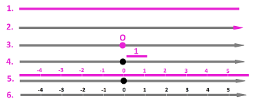
• 1. a line is drawn, the $x$-axis;
• 2. one of the two direction on the line is chosen as positive, then the other is negative;
• 3. a point $O$ is chosen as the origin;
• 4. a segment of the line is chosen as the unit of length;
• 5. the segment is used to measure distances to locations from the origin $O$ -- positive in the positive direction and negative in the negative direction -- and add marks to the line, the coordinates, later the segments are further subdivided to fractions of the unit, etc.

The result looks similar to a ruler:

The idea is to use this set-up to produce a correspondence:

• location $P\ \longleftrightarrow\ $ number $x$,

that works in both directions.

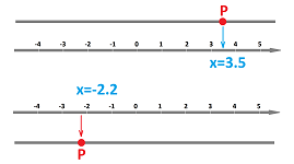
For example, suppose $P$ is a location on the line. We then find the distance from the origin -- positive in the positive direction and negative in the negative direction -- and the result is the coordinate of $P$, some number $x$. We use the nearest mark to simplify the task.

Conversely, suppose $x$ is a number. We then measure $x$ as the distance to the origin -- positive in the positive direction and negative in the negative direction -- and the result is a location $P$ on the line. We use the nearest mark to simplify the task.

Note that we started integers and then also included fraction, i.e., rational numbers. However, we then realize that some of the locations have no counterparts among these numbers. That's how the irrational numbers -- $\sqrt{2},\ \pi$, etc. -- come into play. Together they constitute the real numbers. Then this $1$-dimensional coordinate system is called the real number line or simply the number line. It is also called the $x$-axis.

Definition. The coordinate $x$ of a point $P$ on the $x$-axis is the signed distance from $O$ to $P$, i.e., $x>0$ when $P$ is to the right of $O$ and $x<0$ when $P$ is to the left of $O$.

Once the coordinate system is in place, it is acceptable to think of location as numbers and vice versa. In fact, we can write: $$P=x.$$

Now that everything is pre-measured we can solve the geometric problems by algebraically manipulating coordinates.

Let's consider the first geometric task, distance. We introduce two concepts describing how far apart locations $P$ and $Q$ are.

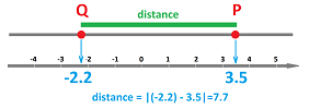
Definition. The signed distance from location $P$ to location $Q$ is the difference of their coordinates; i.e., if $P$ and $Q$ are given by their coordinates $x$ and $x'$, then the distance from $P$ to $Q$ is $$x'-x.$$

Thus, the order matters! The signed distance from $x$ to $x'$ is

• positive when $x<x'$,
• negative when $x>x'$.

The signed distance from $P$ to $Q$ is not the same as the signed distance from $Q$ to $P$. In fact, one is the negative of the other: $$x-x'=-(x'-x).$$

The next definition is meant to erase this difference.

Definition. The unsigned distance between locations $P$ and $Q$ given by their coordinates $x$ and $x'$ is

• $x'-x$ when $x<x'$,
• $x-x'$ when $x>x'$.

Thus, the order doesn't matter! Furthermore, the unsigned distance between two locations is always positive unless the locations coincide.

The word “unsigned” is typically omitted.

Fortunately, we have the absolute value to provide us with a single formula.

Theorem (Distance Formula for dimension $1$). The distance between points with coordinates $x$ and $x'$ is $$|x-x'|.$$

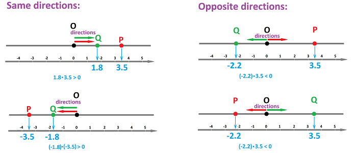
Now the second geometric task, directions. What is the difference between the directions from the origin $O$ toward locations $P$ and $Q$ (other than $O$) represented in terms of their coordinates $x$ and $x'$? There can be only two possibilities:

• if $P$ and $Q$ are on the same side of $O$ then the directions are the same,
• if $P$ and $Q$ are on the opposite sides of $O$ then the directions are the opposite.

Now algebraically,

• if $x>0,\ x'>0$ or $x<0,\ x'<0$ then the directions are the same,
• if $x>0,\ x'<0$ or $x<0,\ x'>0$ then the directions are the opposite.

Fortunately, the product provides us with a single expression.

Theorem (Directions for dimension $1$). The directions from $O$ to $x\ne 0$ and $x'\ne 0$ are

• the same if $x\cdot x'>0$; and
• the opposite if $x\cdot x'<0$.

Exercise. Express the directions in terms of the signed distance.

Since the result is entirely about the signs of these numbers, it can be restated in terms of the sign function: $$\operatorname{sign}(a)=\begin{cases} -1&\text{ if } a<0,\\ 0&\text{ if } a=0,\\ 1&\text{ if } a>0. \end{cases}$$ For $a\ne 0$, it can also be computed by the formula: $$\operatorname{sign}(a)=\frac{a}{|a|}.$$ Thus, the directions from $O$ to $x\ne 0$ and $x'\ne 0$ are

• the same if $\operatorname{sign}(x)= \operatorname{sign}(x')$; and
• the opposite if $\operatorname{sign}(x)\ne \operatorname{sign}(x')$.

The coordinate system for dimension $2$

We continue with dimension $2$. There is much more going on:

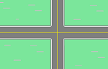
Suppose we live on a field with two roads intersecting surrounded by nothing.

The coordinate system intended to capture what happens on this field is devised to be superimposed on the field.

It is built in several stages:

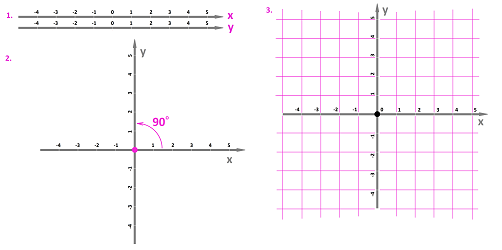
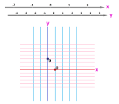
• 1. two coordinate axes are chosen, the $x$-axis first and the $y$-axis second;
• 2. the two axes are put together at their origins so that it is a $90$-degree turn from the positive direction of the $x$-axis to the positive direction of the $y$-axis;
• 3. use the marks on the axis to draw a grid.

The idea is to use this set-up to produce a correspondence:

• location $P\ \longleftrightarrow\ $ a pair of numbers $(x,y)$.

that works in both directions.

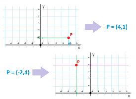
For example, suppose $P$ is a location on the plane. We then find the distances from either of the two axes to that location -- positive in the positive direction and negative in the negative direction -- and the result is the two coordinates of $P$, some numbers $x$ and $y$. We use the nearest mark to simplify the task.

Conversely, suppose $x$ and $y$ are numbers. First, we measure $x$ as the distance from the $y$-axis -- positive in the positive direction and negative in the negative direction -- and such locations together form a vertical line. Second, we measure $y$ as the distance from the $x$-axis -- positive in the positive direction and negative in the negative direction -- and such locations together form a horizontal line. The intersection of these two lines is a location $P$ on the plane. We use the nearest marks to simplify the task.

This $2$-dimensional coordinate system is called the Cartesian plane or the $xy$-plane.

Once the coordinate system is in place, it is acceptable to think of location as pairs of numbers and vice versa. In fact, we can write: $$P=(x,y).$$

Example. Visible uses of the $2$-dimensional Cartesian system aren't as widespread as those for dimension $1$. They are however common in the digital, computing environment.

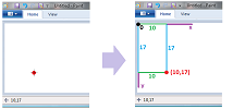
For example, drawing applications, such as Microsoft Paint, allow you to make use of this system -- if you understand it. The location of your mouse is shown in the status bar on the lower left, constantly updated in real time. Then main difference is that the origin is in the left upper corner of the image and the $y$-axis is pointing down:

The choice is explained by the way we write: downward.

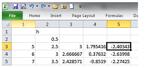
Similarly, spreadsheet applications, such Microsoft Excel, use the Cartesian system (also starting at the upper right corner) to provide a convenient way of representing locations of cells:

This is very important for expressing a value located in one cell in terms of values located in other cells -- via formulas. $\square$

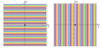
One can think of the $xy$-plane as a stack of lines, vertical or horizontal, each of which is just a copy of one of the axes:

We can use this idea to reveal the internal structure of the coordinate plane.

Theorem.

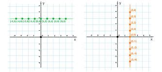
• (a) If $L$ is a line parallel to the $x$-axis, then all points on $L$ have the same $y$-coordinate. Conversely, if a collection $L$ of points on the $xy$-plane consists of all points with the same $y$-coordinate, $L$ is a line parallel to the $x$-axis.
• (b) If $L$ is a line parallel to the $y$-axis, then all points on $L$ have the same $x$-coordinate. Conversely, if a collection $L$ of points on the $xy$-plane consists of all points with the same $x$-coordinate, $L$ is a line parallel to the $y$-axis.

Then, we have a compact way to represent these lines:

• horizontal: $y=k$, and
• vertical: $x=k$,

for some real $k$.

Now that everything is pre-measured we can solve the geometric problems by algebraically manipulating coordinates.

Let's consider the first geometric task, distance. What is the distance between locations $P$ and $Q$ in terms of their coordinates $(x,y)$ and $(x',y')$? The idea is to use the distance formula from the $1$-dimensional case for either of the two axis!

The distance

• between $x$ and $x'$ on the $x$-axis is $|x-x'|$, and
• between $y$ and $y'$ on the $y$-axis is $|y-y'|$.

Then, the segment between the points $P(x,y)$ and $Q=(x',y')$ is the hypotenuse of the right triangle with sides: $|x-x'|$ and $|y-y'|$.

Then our conclusion below follows from the Pythagorean Theorem.

Theorem (Distance Formula for dimension $2$). The distance between points with coordinates $(x,y)$ and $(x',y')$ is $$\sqrt{(x-x')^2+(y-y')^2}.$$

In particular we have the distance to the origin from $(x,y)$ denoted by: $$|(x,y)|=\sqrt{x^2+y^2}.$$

Now the second geometric task, directions. What is the difference between the directions from the origin $O$ toward locations $P$ and $Q$ (other than $O$) represented in terms of their coordinates $(x,y)$ and $(x',y')$? We are talking about angle between the two directions.

Let's first consider the simpler case when $Q=(1,0)$. Then angle the line $OP$ makes with the $x$-axis is fully determined from trigonometry by the coordinates of $P=(x,y)$.

Theorem (Slope). The angle $\alpha$ between the $x$-axis and the line from $O$ to $P=(x,y)\ne O$ is given by its slope: $$\tan \alpha =\frac{y}{x}.$$

Similarly, from the same triangle, in the general case we have the following for the two angles from the $x$-axis to $P$ and to $Q$ respectively: $$\begin{array}{lll} \cos \alpha =\frac{x}{\sqrt{x^2+y^2}},& \cos \beta =\frac{x'}{\sqrt{{x'}^2+{y'}^2}};\\ \sin \alpha =\frac{y}{\sqrt{x^2+y^2}},& \sin \beta =\frac{y'}{\sqrt{{x'}^2+{y'}^2}}. \end{array}$$

We then use this trigonometric identity: $$\begin{array}{lll} \cos(\alpha - \beta) &= \cos \alpha \cos \beta + \sin \alpha \sin \beta\ \\ &=\frac{x}{\sqrt{x^2+y^2}}\frac{x'}{\sqrt{{x'}^2+{y'}^2}}+\frac{y}{\sqrt{x^2+y^2}}\frac{y'}{\sqrt{{x'}^2+{y'}^2}}\\ &=\frac{xx'+yy'}{\sqrt{x^2+y^2}\sqrt{{x'}^2+{y'}^2}}. \end{array}$$ This formula can be simplified with the so-called dot product defined by: $$(a,b)\cdot(c,d)=ac+bd,$$ and the distance formula above.

Theorem (Directions for dimension $2$). The angle between the lines $OP$ and $OQ$, where $P=(x,y)\ne O$ and $Q=(x',y')\ne O$, is given by: $$\cos \widehat{QOP}=\frac{(x,y)\cdot (x',y')}{|(x,y)||(x',y')|}.$$

Note that when both points are on the $x$-axis, i.e., $y=y'=0$, the formula turns into: $$\cos \widehat{QOP}=\frac{xx'}{|x||x'|}=\frac{x}{|x|}\frac{x'}{|x'|}=\operatorname{sign}(x)\cdot \operatorname{sign}(x').$$ There only two possibilities here, $1$ or $-1$, and, therefore, $\widehat{QOP}$ is either $0$ or $180$ degrees. We thus have recovered the theorem about the directions of lines in dimension $1$!

It is entirely possible to have the $x$-axis measured in miles and the $y$-axis in kilometers! Such a coordinate system would look like this:

When this is the case, the geometric formulas above won't be applicable but one can still speak of a point located “$2$ miles east and $5$ kilometers north” from here. Furthermore, $x$ and $y$ will represent in this study quantities of arbitrary nature:

• time vs. location;
• location vs. weight;
• weight vs. temperature, etc.

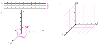
We postpone the $3$-dimensional case until later, but it should be obvious that the construction will start this way:

• 1. build three coordinate axes, ...

and the correspondence will be:

• location $P\ \longleftrightarrow\ $ a triple of numbers $(x,y,z)$.

One can already see how harder is to visualize things in the $3$-dimensional space, which further justifies the need for the algebraic treatment of geometry that we have presented.

How relations and functions emerge...

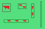
Problem. A farmer with $100$ yards of fencing material wants to build as large a rectangular enclosure as possible for his cattle.

We initially decide to rely entirely on middle school math.

Recalling some geometry, we realize that “the largest enclosure” means the one with the largest area. Now what are the best dimensions?

Trial and Error.

We start to randomly choose possible dimensions of the enclosure and compute their areas:

• $20$ by $20$ gives us the area of $400$ square yards,
• $20$ by $30$ gives us the area of $600$ square yards,
• $20$ by $40$ gives mus the area of $800$ square yards...

It's getting better and better! But wait... $30$ by $30$ gives us $900$! We need to collect more data. Let's speedup this process with a spreadsheet.

Collecting data in a spreadsheet.

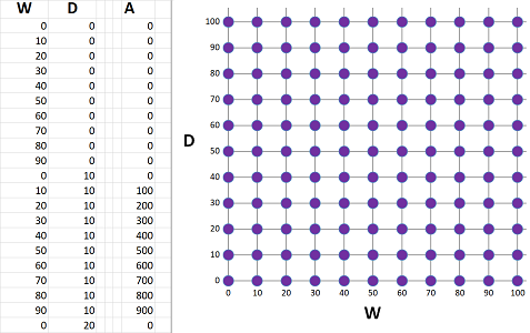
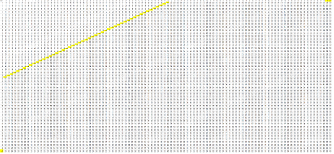
We list all possible combinations -- every $10$ yards -- of a width, column $W$, and depth, column $D$. Both run through these $10$ values: $$W=10,20,...,100 \quad D=10,20,...,100.$$ Together, they form a $10\times 10$ square of possible combinations (plotted in the middle). The last column, $A$, contains the area of each choice of dimensions. It is computed as: $$A=W\cdot D.$$

In the plot on far right, we list the $10$ possible values of the width $W$ and then plot above that value the areas of all possible enclosures -- as the depth increases.

We can see that it's getting better and better as we increase the width or depth. But wait... the perimeter of a $20\times 40$ enclosure is $20+20+40+40=120$. Not enough fencing! Also, the $20 \times 20$ enclosure seems useless too as it doesn't use all the fencing material...

We need to test whether a given combination of width and depth uses exactly $100$ yards of the fencing material. First, we choose to test each dimension every single yard: $$W=1,2,...,100 \quad D=1,2,...,100.$$ We have then $100\cdot 100=10,000$ possible combinations. We also add another column, $P$, for the perimeter computed as: $$P=2( W + D ).$$ We can now check whether such an enclosure satisfies $P=100$ and then plot this point if does. This is called a relation: two variable numbers $W$ and $D$ are related if $2( W + D )=100$.

What we have to test, to be precise, isn't the exact equality $P=100$ but test whether it is a good enough approximation, within $1$ yard: $$99<P<101.$$

Let's examine the plots.

• First, the allowed pairs of dimensions, $(W,D)$, don't form a square anymore but a strip.

This is another relation: two numbers $W$ and $D$ are related if $99<2( W + D )<101$.

• Second, the areas of these allowed pairs seem to form curves.

They seem to indicate that the best choice of a width is somewhere between $20$ and $30$.

There must be a better way...

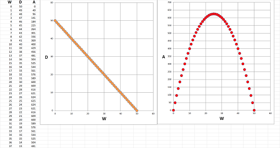
What if we represent this relation explicitly? What if we express $D$ in terms of $W$? It is simple, with middle school algebra. If we start with $2( W + D )=100$, conclude: $$D=50-W.$$ Such an implicit relation between two variables is called a function. This is the data: $$\begin{array}{l|lll} W&L\\ \hline 10&40\\ 20&30\\ 30&20\\ 40&10\\ 50&0 \end{array}$$ Only $5$ pairs of we take it $10$ yards at a time. If it's $1$ yard at time, we have $50$. We put those in a new spreadsheet. The first column is for the width $W$ running through: $1,2,...,50$. The second is for the depth $D$, evaluated by $D=50-W$. What's left a whole square of pairs is just a segment:

The areas are also evaluated as before and plotted for each width.

Looking at our plot, $W=25$ seems to be a clear choice. The corresponding area is $A=25\cdot 25=265$ square yards.

Unfortunately, the plot has gaps! What if there is such a width that it gives us the area bigger than $625$?

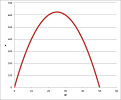
We can see a new function on this spreadsheet: $A$ depends on $W$. With algebra, we have it explicit: $$A=W(50-W).$$ We can restate the problem as $$A=-W^2+50W, \text{ find the largest possible values of } A.$$

Later, we will use the tools of calculus. This time we just use the fact that this is a parabola. What do we know about this curve?

A parabola has a vertex. Because we have “$-$” in the formula for $A$, this one opens down; therefore, we see the desired point in the middle. Where is this point? Parabolas are symmetric; therefore, this point lies the half-way between the two points on the $x$-axis. In our case, those are $0$ and $50$. Therefore, the vertex of the parabola is at $$ x = \frac{ 0 + 50 }{ 2 } = 25. $$

Exercise. Modify the kind of enclosures required by the problem: semicircles are attached to the rectangles, and solve it.

We've solved the problem but we know much less about other, more complicated functions. Calculus will help...

From relations to functions

A relation processes a pair of numbers $(x,y)$ as the input and produces an output, which is: a point or no point; for example: $$ \newcommand{\ra}[1]{\!\!\!\!\!\xrightarrow{\quad#1\quad}\!\!\!\!\!} \newcommand{\da}[1]{\left\downarrow{\scriptstyle#1}\vphantom{\displaystyle\int_0^1}\right.} % \begin{array}{ccccccccccccccc} \text{input} & & \text{relation} & & \text{output} \\ (x,y) & \mapsto & \begin{array}{|c|}\hline\quad x+y=2? \quad \\ \hline\end{array} & \ra{Yes} & \text{ plot } (x,y)\\ &&\downarrow ^{No}\\ &&\text{ don't plot } \end{array}$$ We can do it by hand:

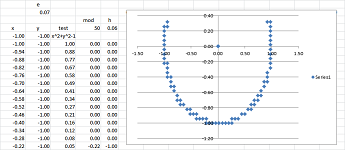
Example. Let's consider something more complex: $$ \newcommand{\ra}[1]{\!\!\!\!\!\xrightarrow{\quad#1\quad}\!\!\!\!\!} \newcommand{\da}[1]{\left\downarrow{\scriptstyle#1}\vphantom{\displaystyle\int_0^1}\right.} % \begin{array}{ccccccccccccccc} \text{input} & & \text{relation} & & \text{output} \\ (x,y) & \mapsto & \begin{array}{|c|}\hline\quad x^2+y^2=1? \quad \\ \hline\end{array} & \ra{Yes} & \text{ plot } (x,y)\\ &&\downarrow ^{No}\\ &&\text{ don't plot } \end{array}$$ We test each of these pairs of $(x,y)$ with help of a spreadsheet:

The formula for the $x$-coordinate is: $$\texttt{ =IF(ABS(RC[-1])<R6C5,RC[-3],0)}.$$ The result looks like a circle. Indeed, $x^2+y^2$ is the square of the distance from $(x,y)$ to the origin. $\square$

Theorem. The circle of radius $R>0$ centered at point $(h,k)$, which is the collection of points $R$ units away from $(h,k)$, is given by the relation: $$(x-h)^2+(y-k)^2=R^2.$$

Proof. It follows from the Distance Formula. $\blacksquare$

Even with a computer, this is like looking for a needle in a haystack. Functions allow us to produce “allowed” pairs $(x,y)$ automatically, without needing to test each of them. Simply plug in a value, $x$, and the function will produce its mate, $y$.

Functions can be illustrated as flowcharts:

$$ \newcommand{\ra}[1]{\!\!\!\!\!\xrightarrow{\quad#1\quad}\!\!\!\!\!} \newcommand{\da}[1]{\left\downarrow{\scriptstyle#1}\vphantom{\displaystyle\int_0^1}\right.} % \begin{array}{ccccccccccccccc} x & \mapsto & \begin{array}{|c|}\hline\quad x+3 \quad \\ \hline\end{array} & \mapsto & y & \mapsto & \begin{array}{|c|}\hline\quad y\cdot 2 \quad \\ \hline\end{array} & \mapsto & z & \mapsto & \begin{array}{|c|}\hline\quad z^2 \quad \\ \hline\end{array} & \mapsto & u \end{array}$$ Note how the names of the variables match, so that we can proceed to the next step. An algebraic representation of the process is: $$y=x+3,\quad z=y\cdot 2,\quad u=z^2.$$

In general, we represent a function diagrammatically as a black box that processes the input and produces the output: $$ \newcommand{\ra}[1]{\!\!\!\!\!\xrightarrow{\quad#1\quad}\!\!\!\!\!} \newcommand{\da}[1]{\left\downarrow{\scriptstyle#1}\vphantom{\displaystyle\int_0^1}\right.} % \begin{array}{ccccccccccccccc} \text{input} & & \text{function} & & \text{output} \\ x & \mapsto & \begin{array}{|c|}\hline\quad f \quad \\ \hline\end{array} & \mapsto & y \end{array}$$ Here, $f$ is the name of the function. In this example, we use a letter to indicate an abstract function while in the examples below functions may be specific with specific names: $$\sqrt{(\quad)},\ \exp (\quad ),\ \sin (\quad ),\ \text{ etc.}$$

Functions come from many sources and can be expressed in different forms:

• an algebraic formula or formulas;
• a table of values;
• a graph;
• an algorithm.

An algebraic formula is exemplified by $y = x^{2}$. In order to properly introduce this as a function, we give it a name, say $f$, and write: $$f(x)=x^2.$$ Here, we are using the following notation: $$\begin{array}{r|ccccccc} &y&=&f&( &x&)&=&x^2\\ &\uparrow&&\uparrow&&\uparrow&&&\uparrow\\ \text{name: }&\text{dependent }&&\text{function }&&\text{independent }&&&\text{independent}\\ &\text{variable }&&\text{ }&&\text{variable }&&&\text{variable} \end{array}$$

Moreover, “piece-wise defined functions” use by several formulas at the same time. The most important one is the following.

Definition. The absolute value function $$f(x) = |x|$$ is computed as follows:

• if $x < 0$ then $y = - x$; and
• if $x \geq 0$ then $y = x$.

We can re-write this algebraically as $$ f(x) = \begin{cases} -x & \text{ if } x < 0, \\ x & \text{ if } x \geq 0. \end{cases} $$

A frequently used property of the absolute value function is the following.

Theorem (Triangle Inequality). For any two numbers $a,b$, we have: $$|a+b|\le |a|+|b|.$$

Proof. $\blacksquare$

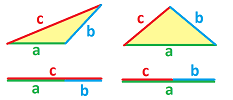
The name of the theorem comes from a similar property of the lengths of the sides of a triangle $a,b,c$: $$|c|<|a|+|b|.$$

When the triangle degenerates into a segment, we have the triangle inequality for numbers.

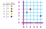
A function can also be represented by a table of values. Such a table has two columns, for $x$ and $y$: $$\begin{array}{l|ll} x&y=f(x)\\ \hline 0&1\\ 1&3\\ 2&4\\ 3&0\\ 4&2\\ ...&... \end{array}$$ This is a numerical representation as the table contains only numbers. Any table would do as long as there are no repetitions in the $x$-column!

To create larger tables, one uses a spreadsheet.

Then each value in the $y$-column is computed from the corresponding value in the $x$-column via some formula. For example, for $y=x^2$, we write in the $y$-column the following: $$\texttt{=RC[-1]^2}.$$

Even though the data in the table represents the same function as above, as we can see, there are gaps in the data. We can't tell, for example, what $1.5^2$ is or what $100^2$ is. Thus, our algebraic representation is complete but the numerical representation given by the table is not.

The advantage of numerical representation is that it has been calculated for you so that you can see patterns; for example,

• if $x$ is increasing, then $y$ is increasing;
• if $x$ grows faster, $y$ also grows faster, etc.

We can use the table data to plot points, which leads us to the graphical representation.

Definition. The graph of a function $f$ is the set of points in the $xy$-plane that satisfy $y=f(x)$. In other words, it is the set of all possible points $$(x,f(x)).$$

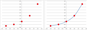
For example, we can plot the above table; just the points that have been provided:

Meanwhile, spreadsheet software comes with graphic capabilities. It will plot all points you have in the table:

It can also automatically add a curve connecting these points.

Note that when $x$ and $y$ represent to variable that have nothing to do with each other -- such as time and location -- neither so the two axes:

An algorithm is a verbal representation of a function. It may contain no algebra. Instead it tells us how to get a certain output given a any given input.

For example,

• Question: How do we get from $x$ to $y$?
• Answer: Let $y$ be equal to the square of $x$.

This representation also gives us compete information about the function.

Example. Describe what this function do: $$f(x)=\dfrac{x^{2} + 1}{x^{2} -1},$$ verbally:

• Step 1: multiply $x$ by itself, call it $y$;
• Step 2: add 1 to $y$, call it $z$;
• Step 3: subtract 1 from $y$, call it $u$;
• Step 4: divide $z$ by $u$.

$\square$

An algorithm can be used to create a computer program. In this case, $x$ is the input, it passes through a black box and out comes $y$. But we must be careful. If our algorithm requires the computer to divide by $x$ and we give it $x=0$, there will be trouble.

Example. Let $$y = f(x) = |x|.$$ Given an input of $x$, describe a procedure for computing this function.

Alternative to the definition given above, we have:

• Step 1: determine the sign, $s=\operatorname{sign}(x)$, of $x$: if $x \geq 0$, then $s = 1$; else $s = -1$;
• Step 2: multiply $x$ by $s$.

We can express this numerically: $$\begin{array}{r|ll} x&y=|x|\\ \hline -3&3\\ -2&2&\text{ decreasing?}\\ -1&1&\text{ decreasing?}\\ 0&0\\ 1&1&\text{ increasing?}\\ 2&2&\text{ increasing?}\\ 3&3\\ \end{array}$$

We do notice some patterns but we would need more points to be sure of the trends. In that case, we can plot all those points and then possibly connect them into a single curve:

$\square$

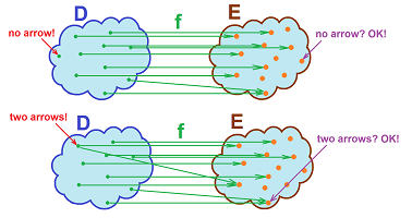
Definition. A function is a rule or procedure $f$ that assigns to any number $x$ in a set $D$, called the domain, one number $y$ in another set of real numbers $E$.

In other words,

• each $x$ in $D$ has a counterpart in $E$, and
• there is only one such counterpart.

This rule can be violated when there are too few or too many arrows for a given $x$:

Then this is not a function. It is OK, however, to have too few or too many arrows for a given $y$!

Algebraically, we plug $x$ into the formula and see if it works.

Example. Let $$ f(x) = \frac{1}{x} .$$

Try $x = 0$. The formula doesn't work because $\frac{1}{0}$ is undefined. If we keep trying, we realize that $\dfrac{1}{x}$ is defined for all $x \neq 0$. Then, we can choose the domain to be all these numbers: $$D_1 = ( - \infty, 0 ) \cup ( 0, +\infty). $$

What about $$D_{2} = (0, \infty )?$$ It is also a valid choice.

The domain may be also $$D_3 = [1,2].$$ $\square$

What is the advantage of one domain over another?

Definition. The largest possible domain for a given formula is called the implied domain (or the natural domain).

Example. Let $$f(x) = \dfrac{x^{2} + 1}{x^{2} - 1},$$ find the implied domain. We need to ensure that the input $x$ doesn't produce a $0$ in the denominator. Solve $$x^{2} - 1 = 0.$$ We see that $x^{2} = 1$. Thus $x = -1$ and $x = + 1$. The function is defined by all values except $\pm 1$, or $$D = ( \infty, -1 ) \cup (-1 , 1) \cup ( 1, \infty).$$ $\square$

These are some “problematic” algebraic operations:

• division (possibly by $0$),
• even degree roots (of possibly negative numbers).

Next, let's revisit the the rule -- how to get $y$ from $x$ -- that defines a function. It must satisfy: there is only one $y$ for each $x$.

Let's illustrate how the rule might fail for each of the four representations of $f$.

$\bullet$ Algebraic: $$y=\pm x.$$

$\bullet$ Numerical: $$\begin{array}{rlr|lll} &&x&y\\ \hline &&...&...\\ &&0&22\\ &\nearrow&...&...&\nwarrow\\ \text{same!}&&...&...&&\text{different!}\\ &\searrow&...&...&\swarrow\\ &&0&55\\ &&...&... \end{array}$$

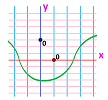
$\bullet$ Graphical:

$\bullet$ Algorithmic:

• Step 1: ...
• ...
• Step 50: add today's date to the output of step 49.
• ...
• Step 100: ...

Then we might face these outcomes: $$\begin{array}{lll} x = 10 &\Longrightarrow &y = 20, \\ &&y = 21, \\ &&y = 22. \end{array} $$

For the graphical representation, all it takes is a glance.

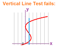
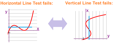
Theorem (Vertical Line Test). A relation is a function if and only if every vertical line crosses the graph at one point or less.

Example. $\square$

Elementary functions

A linear functions is commonly represented by its slope-intercept form: $$\begin{array}{lll} f(x) = & m&\cdot &x & +&b \\ & \uparrow &&&& \uparrow \\ & \textrm{slope} &&&& y\textrm{-intercept} \end{array}$$

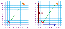
Recall, that the slope of a line is found by choosing two points on the line in a specified order, say, $A$ then $B$. Then, by definition, we have: $$\text{slope } =\frac{\text{rise}}{\text{run}}.$$ The exact meaning of the numerator and denominator is the following.

If we know the coordinates of the points, $$A=(a_1,a_2),\quad B=(b_1,b_2),$$ the slope is computed by: $$m=\frac{\text{signed distance from }a_2 \text{ to } b_2}{\text{signed distance from }a_1 \text{ to } b_1}.$$ The result is, of course, the same if we reverse the order: $B$ first, $A$ second. Indeed, both numerator and denominator simply change their signs: $$m=\frac{\text{signed distance from }b_2 \text{ to } a_2}{\text{signed distance from }b_1 \text{ to } a_1}.$$

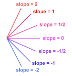
We can arrange all linear functions according to their slopes:

Monotonicity of linear functions is easy to determine:

• $m > 0\ \Longrightarrow\ f$ is increasing, on the whole domain.
• $m < 0\ \Longrightarrow\ f$ is decreasing, on the whole domain.
• $m = 0\ \Longrightarrow\ f$ is constant, on the whole domain.

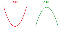
A quadratic functions is presented in the standard form: $$ f(x) = ax^{2} + bx + c, \ a\ne 0. $$ We know that

• if $a > 0$, parabola opens up;
• if $a < 0$, parabola opens down.

Note: the case $a = 0$ is linear not quadratic.

The domain is all reals.

Proposition. The $x$-coordinate of the vertex of parabola (i.e., max or min) is $$ v = - \frac{b}{2 a }. $$

Proposition. $$ y = - \frac{b}{2 a } $$ is the equation of the axis of the parabola.

As building block for future more complex functions, we introduce the (positive) power functions : $$ \underbrace{x^{0} = 1}_{\text{constant}}, \underbrace{x}_{\text{linear}}, \underbrace{x^{2}}_{\text{quadratic}}, \underbrace{x^{3}}_{\text{cubic}}, \cdots , \underbrace{x^{n}}_{n\text{th degree}}, ... $$ Beyond the first few, we use the power of $x$, called the degree, to identify these functions.

The domains are all real numbers.

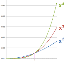
The magnitude of the degree affects the shape of the graph:

The higher the degree, the slower the graph grows from $x=0$ and the faster it rises from $x=1$. They all meet at $(1,1)$.

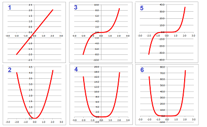
We can see a pattern below:

In the first row, the graphs look like parabolas (with flatter bottom). These are ever powers. When the power is odd, the graphs look like $x^{3}$. Thus, the parity of degree, i.e., odd vs. even, significantly affects the shape of the graph.

In addition to the positive power functions, we introduce the negative power functions as the reciprocals of the former: $$x^{-1}=\frac{1}{x^1},\ x^{-2}=\frac{1}{x^2},\ x^{-3}=\frac{1}{x^3},\ ....,\ x^{-n}=\frac{1}{x^n},... $$ Their domains are the same: $(-\infty,0)\cup(0,+\infty)$.

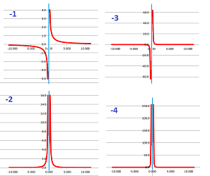
The magnitude of the degree affects the shape of the graph:

The higher the degree, the faster the graph drops from $x=0$ and the slower it declines from $x=1$. They all meet at $(1,1)$.

Monotonicity

When we say that a function increases, we mean that the graph rises and we say it decreases when its graph drops:

This verbal definition is simple and the geometric meaning is very clear. However, both are imprecise. Even though we understand increasing functions as ones with graphs rising and decreasing functions as one with graphs falling, the precise definition has to rely on considering one pair of points at a time.

Definition. A function $y=f(x)$ is called increasing on interval $(A,B)$ if $$f(a)<f(b) \text{ for all } A<a<b<B;$$ a function $y=f(x)$ is called decreasing on interval $(A,B)$ if $$f(a)>f(b) \text{ for all } A<a<b<B.$$ The function is also called non-decreasing and non-increasing respectively if we replace the strict inequality signs “$<$” and “$>$” with non-strict “$\le $” and “$\ge $”.

Example. Note that a constant function is both non-decreasing and non-increasing but neither decreasing nor increasing. $\square$

How do we verify these conditions? Let's work out some examples algebraically.

Example. We utilize what we know about the algebra of inequalities.

First, we can multiply both sides of an inequality by a positive number: $$a<b\ \Longrightarrow\ 3a<3b.$$ Therefore, the function $f(x)=3x$ is increasing.

Second, if we multiply both sides of an inequality by a negative number, we have to reverse the sign: $$a<b\ \Longrightarrow\ (-2)a>(-2)b.$$ Therefore, the function $f(x)=-2x$ is decreasing.

Third, we can add any number to both sides of an inequality: $$a<b\ \Longrightarrow\ a+4<b+4.$$ Therefore, the function $f(x)=x+4$ is increasing. $\square$

Putting these facts together, we acquire the following.

Theorem. A linear function $$f(x)=mx+b$$

• is increasing if $m>0$, and
• is decreasing if $m<0$.

Example. This is how we can solve this problem one function at a time, from scratch. Let $$ f(x) = 3x - 7. $$ If $x_{1} < x_{2}$ then $$\begin{array}{rrclcc} f(x_{1}) = &3 x_{1} - 7 & \overset{?}{<} &f(x_{2}) = 3 x_{2} - 7 \\ \Longrightarrow &3 x_{1} & \overset{?}{<}& 3 x_{2} \\ \Longrightarrow &x_{1} & < &x_{2}. \end{array}$$ The computation suggests that $y=f(x)$ is increasing. For a complete proof, retrace these steps backwards. $\square$

Things get harder for quadratic, cubic,... functions as they lead to quadratic, cubic, ... inequalities.

Example. Let's consider $$f(x)=x^2.$$

First, we can multiply two inequalities, when they are aligned and their signs are positive: $$\begin{array}{ll}0<a<b\\ 0<a<b\end{array}\ \Longrightarrow\ 0<a\cdot a <b\cdot b\ \Longrightarrow\ a^2<b^2.$$ Therefore, the function $f(x)=x^2$ is increasing for $x>0$.

Second, if we multiply two inequalities when their signs are negative, we have to reverse the sign: $$\begin{array}{ll}a<b<0\\ a<b<0\end{array}\ \Longrightarrow\ a\cdot a >b\cdot b>0 \ \Longrightarrow\ a^2>b^2.$$ Therefore, the function $f(x)=x^2$ is decreasing for $x<0$. $\square$

Example. Now, we let $$f(x)=x^3,$$ and follow a similar procedure starting with two unknown $a,b$ with $a<b$. We can multiply three identical inequalities -- positive or negative -- and preserve the sign: $$\begin{array}{ll}a<b\\ a<b\\ a<b\end{array}\ \Longrightarrow\ a\cdot a\cdot a <b\cdot b\cdot b\ \Longrightarrow\ a^3<b^3.$$ Therefore, the function $f(x)=x^3$ is increasing for all $x$. $\square$

Notation: We will use

• “$\nearrow$” for increasing, and
• “$\searrow$” for decreasing behavior.

In particular,

• if $f(x)=2x-3$, then $f \nearrow $ on $(-\infty, +\infty)$;
• if $g(x)=-5x+4$, then $g \searrow $ on $(-\infty, +\infty)$;
• if $h(x)=x^2$, then $h \searrow $ on $(-\infty, 0)$ and $\nearrow $ on $(0, +\infty)$;
• if $k(x)=x^3$, then $k \nearrow $ on $(-\infty, +\infty)$.

When a function is either increasing on an interval or decreasing on it, we call it monotonic on the interval.

Polynomials

Definition. A polynomial of degree $n$ is given by a formula: $$ f(x) = a_nx^n+a_{n-1}x^{n-1}+...+a_2x^2+a_1x+a_0, $$ where $a_n,\ a_{n-1},\ ...,\ a_2,\ a_1,\ a_0$ are real numbers called the coefficients of the polynomial, $a_n\ne 0$.

Thus, polynomials are “made” of powers of $x$ via multiplication by the coefficients and then addition: $$x^{3}+x^{2} + 1. $$

Polynomials include all linear and quadratic functions, as well as the power functions.

Example. Let's analyze this polynomial: $$\begin{array}{llll} f(x)&=(x^4-9x^2)(x^2-3)^2&\text{ ...we need to further factor it! }\\ &=x^2(x-3)(x+3)(x-\sqrt{3})^2(x+\sqrt{3})^2. \end{array}$$ With only irreducible factor listed, we can see the $x$-intercepts. They are simply read off the list of factors: $$x=0,\ 3,\ -3,\ -\sqrt{3},\ \sqrt{3}.$$ At these points and at these points only the function may change its sign. We now list all the factors. They are simple enough for us to determine where and whether they change their signs: $$\begin{array}{l|cccccccccc} \text{factors }& \text{ signs }\\ \hline x^2&+&+&+&+&+&0&+&+&+&+&+\\ x-3&-&-&-&-&-&-&-&-&-&0&+\\ x+3&-&0&+&+&+&+&+&+&+&+&+\\ (x-\sqrt{3})^2&+&+&+&+&+&+&+&+&+&+&+\\ (x+\sqrt{3})^2&+&+&+&+&+&+&+&+&+&+&+\\ \hline \text{domain }&\cdots&\bullet&\cdots&\bullet&\cdots&\bullet&\cdots&\bullet&\cdots&\bullet&\cdots&\to x\\ x=&&-3&&-\sqrt{3}&&0&&\sqrt{3}&&3\\ \hline f(x)=&+&0&-&0&-&0&-&0&-&0&+\\ &\searrow&0&\smile&0&\smile&0&\smile&0&\smile&0&\nearrow \end{array}$$ Here we went vertically in each column and determined the sign of the function using: $+\cdot-=-$, etc. An idea of what the graph of $f$ looks like is seen in the last row: it crosses the $x$-axis downward, then touches it three times from below, and then crosses it upward. The table solves for us this equation and these inequalities: $$f(x)=0,\ f(x)>0,\ f(x)\ge 0,\ f(x)<0,\ f(x)\le 0.$$ $\square$

Definition. Function $f$ is called rational if $$ f(x) = \frac{P(x)}{Q(x)}, $$ where $P$ and $Q$ are polynomials.

They are called this way because they are ratios of polynomials: $$ \left. \frac{ x^2 - 1 }{ x^2 + x-1 } \right\} \text{ two polynomials } $$

How do we find the implied domain of a rational function?

Example. What is the domain of $$f(x)=\dfrac{x - 1}{x + 1}?$$ Solution: We look at the denominator, set it equal to zero, $x + 1 = 0$, and solve. Then $x = -1 $ is not in the domain and the rest of the real numbers are. $\square$

Example. What is the domain of $$ f(x) = \frac{x - 1}{x^{2} - 4}? $$ Set the denominator to $0$ and solve: $$ \begin{array}{rl} x^{2} - 4 & = 0 \\ x^{2} & = 4 \\ x & = \pm 2 \end{array} $$ So the domain consists of all real numbers except $\pm 2$. $\square$

Example. Let's analyze this rational function: $$f(x) = \frac{x(3x^{2} + 1)}{(x-1)(x+1)}.$$ First, the domain is all reals except $x=\pm 1$. We now need find the signs of the factors and then the signs of the function. We take note of the domain and only list the factors that may change sign ($(3x^{2} + 1)$ can't): $$\begin{array}{l|cccccccccc} \text{factors }& \text{ signs }\\ \hline x&-&-&-&0&+&+&+\\ x-1 &-&-&-&-&-&0&+\\ x+1 &-&0&+&+&+&+&+\\ \hline \text{domain }&\cdots&\circ&\cdots&\bullet&\cdots&\circ&\cdots&\to x\\ x=&&-1&&0&&1&&\\ \hline f(x)&+& &-&0&-& &+\\ \end{array}$$ $\square$

Algebra of functions

For each of the four algebraic operations on numbers -- addition, subtraction, multiplication, and division -- there is an operation on functions.

Functions are transformations of the line

...and vice versa.

We think as if the whole $x$-axis is drawn on a pencil:

We start with a shift. We simply slide the pencil horizontally. Furthermore, there is another pencil to be used for reference. The markings (i.e., its coordinate system) on the second pencil show the new locations of the points on the first. For example, a shift of $3$ units right is shown below:

Generally,

• when shifted $k>0$ units right, point $x$ becomes $x+k$.

In the mean time, what about shift left? We have:

• when shifted $k>0$ units left, point $x$ becomes $x-k$.

Of course, we can combine the two statements:

• when shifted $k>0$ units right/left, point $x$ becomes $x\pm k$.

Instead, we should allow $k$ to be negative. Then we can interpret the former statement to include the latter if we understand “$k$ units left” as “$-k$ units right”. This is a way describe it: $$\newcommand{\ra}[1]{\!\!\!\!\!\xrightarrow{\quad#1\quad}\!\!\!\!\!} \newcommand{\da}[1]{\left\downarrow{\scriptstyle#1}\vphantom{\displaystyle\int_0^1}\right.} \begin{array}{ccc} x& \ra{ \text{ right } k}& x+k. \end{array}$$ This is a function: $$f(x)=x+k.$$

Now a different kind of transformation, flip. We lift, then flip the pencil with $x$-axis on it, and place next to another such pencil. This flip is shown below:

This is the algebraic interpretation: $$\newcommand{\ra}[1]{\!\!\!\!\!\xrightarrow{\quad#1\quad}\!\!\!\!\!} \newcommand{\da}[1]{\left\downarrow{\scriptstyle#1}\vphantom{\displaystyle\int_0^1}\right.} \begin{array}{ccc} x& \ra{ \text{ flip } }& -x. \end{array}$$ This is another function: $$f(x)=-x.$$

A new type of transformation is a stretch. The line isn't on a pencil anymore! It is a rubber string with knots:

We grab it by the ends and pull them apart in such a way that the origin doesn't move. For example, a stretch by a factor of $2$ is shown below:

Generally,

• when the line is stretched by a factor $k>1$, point $x$ becomes $x\cdot k $.

In the mean time, what about a shrink? We have:

• when the line is shrunk by a factor $k>1$, point $x$ becomes $x/k$.

Of course, in order to combine the two statements, we should allow $k$ to be less than $1$. Then we can interpret the former statement to include the latter if we understand “stretched by a factor $k$” as “shrunk by a factor $1/k$”. This is a way describe it ($k>0$): $$\newcommand{\ra}[1]{\!\!\!\!\!\xrightarrow{\quad#1\quad}\!\!\!\!\!} \newcommand{\da}[1]{\left\downarrow{\scriptstyle#1}\vphantom{\displaystyle\int_0^1}\right.} \begin{array}{ccc} x& \ra{ \text{ stretch by } k}& x\cdot k. \end{array}$$ This is the third kind of function that we have discovered: $$f(x)=x\cdot k.$$

What about the $y$-axis? Then the line -- pencil and string -- is vertical. We have a vertical shift: $$\newcommand{\ra}[1]{\!\!\!\!\!\xrightarrow{\quad#1\quad}\!\!\!\!\!} \newcommand{\da}[1]{\left\downarrow{\scriptstyle#1}\vphantom{\displaystyle\int_0^1}\right.} \begin{array}{ccc} y& \ra{ \text{ up } k}& g(y)=y+k; \end{array}$$ a vertical flip: $$\newcommand{\ra}[1]{\!\!\!\!\!\xrightarrow{\quad#1\quad}\!\!\!\!\!} \newcommand{\da}[1]{\left\downarrow{\scriptstyle#1}\vphantom{\displaystyle\int_0^1}\right.} \begin{array}{ccc} y& \ra{ \text{ flip } }& g(y)=-y; \end{array}$$ and a vertical stretch: $$\newcommand{\ra}[1]{\!\!\!\!\!\xrightarrow{\quad#1\quad}\!\!\!\!\!} \newcommand{\da}[1]{\left\downarrow{\scriptstyle#1}\vphantom{\displaystyle\int_0^1}\right.} \begin{array}{ccc} y& \ra{ \text{ stretch by } k}& g(y)=y\cdot k. \end{array}$$

Transformations of the axes produce new functions

We will see how the transformations of the axes -- both horizontal and vertical -- affect the functions.

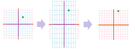
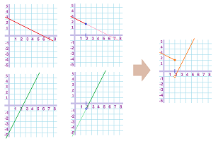
We start with a shift, vertical. We shift the whole $xy$-plane as if it is drawn on a sheet of paper. Furthermore, there is another sheet of paper underneath used for reference. It is on the second sheet that we see the resulting points. We then use its coordinate system to record the coordinates of the new point. For example, a shift of $3$ units upward is shown below:

Generally,

• when shifted $k>0$ units up, point $(x,y)$ becomes $(x,y+k)$.

We understand “$k$ units down” as “$-k$ units up”. This is a way describe it: $$\newcommand{\ra}[1]{\!\!\!\!\!\xrightarrow{\quad#1\quad}\!\!\!\!\!} \newcommand{\da}[1]{\left\downarrow{\scriptstyle#1}\vphantom{\displaystyle\int_0^1}\right.} \begin{array}{ccc} (x,y)& \ra{ \text{ up } k}& (x,y+k). \end{array}$$

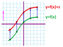
We next apply this operation to study graphs of functions. Since the graph is drawn on the same piece of paper, it is shifted exactly the same way. What about the formula for the new function? Suppose a point $(x,y)$ lies on the graph of $f$, then $f(x)=y$. The shifted point $(x,y+k)$ lies on the graph of the new function $g$, hence $g(x)=y+k=f(x)+k$.

Such a shift can be carried out point by point:

Rule 1 (vertical shift): If the graph $y = g(x)$ is the graph of $y = f(x)$ shifted $k$ units up, then $$ g(x) = f(x) + k, $$ and vice versa.

By “vice versa” we mean that if function $g$ satisfies $g(x) = f(x) + k$ then its graph is the graph of $f$ shifted $k$ units up.

The most important conclusion is the new function has the exact same shape of the graph as the old one.

Example. The graph of each of these: $$x^{2}, x^{2} + 1, x^{2} + 10, x^{2} - 1 , x^{2} - 10,$$ is the same parabola just differently located. $\square$

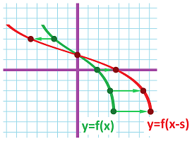
What about the horizontal shift? For example, a shift of $2$ units right is shown below:

We again allow the shift to be negative and understand “$k$ units left” as “$-k$ units right”. This is a way describe it: $$\newcommand{\ra}[1]{\!\!\!\!\!\xrightarrow{\quad#1\quad}\!\!\!\!\!} \newcommand{\da}[1]{\left\downarrow{\scriptstyle#1}\vphantom{\displaystyle\int_0^1}\right.} \begin{array}{ccc} (x,y)& \ra{ \text{ right } k}& (x+k,y). \end{array}$$

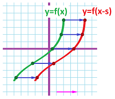
What about the formula for a function shifted this way? Things are a bit more complicated than for a horizontal shift. Suppose a point $(x,y)$ lies on the graph of $f$, then $f(x)=y$. The shifted point $(x+k,y)$ lies on the graph of the new function $g$, hence $g(x+k)=y=f(x)$. Therefore, the new function is $g(x)=f(x-k)$.

Such a shift can be carried out point by point:

Example. Take $f(x) = x^{2}$, and shift $2$ units to the left and to the right too; we get $$ g(x) = f(x+2) = (x+2)^{2} \text{ and } h(x) = f(x-2) = (x-2)^{2}. $$

To confirm the match, what is the $x$-intercept of $g$? Set $g(x) = 0$ and $h(x)=0$, and solve: $$\begin{array}{r | l} (x + 2) ^2 = 0 & (x - 2) ^2 = 0 \\ x + 2 = 0 & x - 2=0 \\ x = -2 & x = 2\\ \text{left shift } & \text{ right shift } \end{array}$$ $\square$

Rule 2 (horizontal shift): If the graph of $g$ is the graph of $f$ shifted $k$ units to the right, then $$ g(x) = f(x-k),$$ and vice versa.

Once again, the new function has the exact same shape of the graph as the old one.

This is the algorithmic interpretation of these shifts. Vertical shift, up $3$ units: $$ \newcommand{\ra}[1]{\!\!\!\!\!\xrightarrow{\quad#1\quad}\!\!\!\!\!} \newcommand{\da}[1]{\left\downarrow{\scriptstyle#1}\vphantom{\displaystyle\int_0^1}\right.} % \begin{array}{ccccccccccccccc} x & \mapsto & \begin{array}{|c|}\hline\quad f \quad \\ \hline\end{array} & \mapsto & u & \mapsto & \begin{array}{|c|}\hline\quad u+3 \quad \\ \hline\end{array} & \mapsto & y; \end{array}$$ horizontal shift, left $2$ units: $$ \newcommand{\ra}[1]{\!\!\!\!\!\xrightarrow{\quad#1\quad}\!\!\!\!\!} \newcommand{\da}[1]{\left\downarrow{\scriptstyle#1}\vphantom{\displaystyle\int_0^1}\right.} % \begin{array}{ccccccccccccccc} x & \mapsto & \begin{array}{|c|}\hline\quad x+2 \quad \\ \hline\end{array} & \mapsto & u & \mapsto & \begin{array}{|c|}\hline\quad f \quad \\ \hline\end{array} & \mapsto & y. \end{array}$$

These shifts can also be described a translation along the $y$-axis and a translation along the $x$-axis respectively. That is why the former only changes the $y$-coordinates of the points and the latter only the $x$-coordinates.

What about combinations of these two transformations?

Example. Let $$h(x) = (x + 2)^{2} +4.$$ What is the graph?

First, analysis: $$ \newcommand{\ra}[1]{\!\!\!\!\!\xrightarrow{\quad#1\quad}\!\!\!\!\!} \newcommand{\da}[1]{\left\downarrow{\scriptstyle#1}\vphantom{\displaystyle\int_0^1}\right.} % \begin{array}{ccccccccccccccc} x & \mapsto & \begin{array}{|c|}\hline\quad x+2 \quad \\ \hline\end{array} & \mapsto & u & \mapsto & \begin{array}{|c|}\hline\quad u^2 \quad \\ \hline\end{array} & \mapsto & z & \mapsto & \begin{array}{|c|}\hline\quad z+4 \quad \\ \hline\end{array} & \mapsto & y \end{array}$$

This is a $2$-unit left shift followed by a $4$-unit up shift.

$\square$

Exercise. What happens to the $x$- and $y$-intercepts of a function under vertical and horizontal shifts?

Exercise. What happens to the domain and the range of a function under vertical and horizontal shifts?

Now a different kind of transformation, flip, vertical. We lift, then flip the sheet of paper with $xy$-plane on it, and finally place it on top of another such sheet so that the $x$-axes align. This flip is shown below:

This is the algebraic outcome: $$\newcommand{\ra}[1]{\!\!\!\!\!\xrightarrow{\quad#1\quad}\!\!\!\!\!} \newcommand{\da}[1]{\left\downarrow{\scriptstyle#1}\vphantom{\displaystyle\int_0^1}\right.} \begin{array}{ccc} (x,y)& \ra{ \text{ vertical flip } }& (x,-y). \end{array}$$

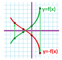
We next apply this operation to study graphs of functions. Since the graph is drawn on the same piece of paper, it is flip exactly the same way. What about the formula for the new function? Suppose a point $(x,y)$ lies on the graph of $f$, then $f(x)=y$. The flipped point $(x,-y)$ lies on the graph of the new function $g$, hence $g(x)=-y=-f(x)$.

Such a flip can be carried out point by point:

Rule 3 (vertical flip): If the graph of $g$ is the graph of $f$ flipped vertically then $$ g(x) = - f(x), $$ and vice versa.

Again, the new function has the exact same shape of the graph as the old one.

Example. Let $$ h(x) = - f(x) + 3. $$ How do we get the graph of $h$? $$ x \longmapsto f(x) \underbrace{\longmapsto}_{\textrm{vertical flip}} - f(x) \underbrace{\longmapsto}_{\textrm{vertical shift}} - f(x) + 3. $$ The order matters... Let's interchange these two: $$ x \longmapsto f(x) \underbrace{\longmapsto}_{\textrm{vertical shift}} f(x) + 3 \underbrace{\longmapsto}_{\textrm{vertical flip}} - (f(x)+3). $$ The graphs are also different:

$\square$

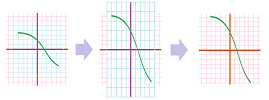
For the horizontal flip, we lift, then flip the sheet of paper with $xy$-plane on it, and finally place it on top of another such sheet so that the $y$-axes align. This flip is shown below:

This is the algebraic outcome: $$\newcommand{\ra}[1]{\!\!\!\!\!\xrightarrow{\quad#1\quad}\!\!\!\!\!} \newcommand{\da}[1]{\left\downarrow{\scriptstyle#1}\vphantom{\displaystyle\int_0^1}\right.} \begin{array}{ccc} (x,y)& \ra{ \text{ horizontal flip } }& (-x,y). \end{array}$$

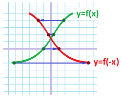
Now, the graphs of functions transformed this way. What about the formula for the new function? Suppose a point $(x,y)$ lies on the graph of $f$, then $f(x)=y$. The flipped point $(-x,y)$ lies on the graph of the new function $g$, hence $g(-x)=y=f(x)$. Therefore, $g(x)=-f(x)$.

Such a flip can be carried out point by point:

Rule 4 (horizontal flip): If the graph of $y = g(x)$ is the graph of $y = f(x)$ flipped horizontally, then $$ g(x) = f(-x), $$ and vice versa.

Exercise. Does the order matter when the horizontal flip is combined with a horizontal shift? What about the horizontal flip with a vertical shift?

Vertical flip: $$ \newcommand{\ra}[1]{\!\!\!\!\!\xrightarrow{\quad#1\quad}\!\!\!\!\!} \newcommand{\da}[1]{\left\downarrow{\scriptstyle#1}\vphantom{\displaystyle\int_0^1}\right.} % \begin{array}{ccccccccccccccc} x & \mapsto & \begin{array}{|c|}\hline\quad f \quad \\ \hline\end{array} & \mapsto & u & \mapsto & \begin{array}{|c|}\hline\quad -u \quad \\ \hline\end{array} & \mapsto & y \end{array}$$ Horizontal flip: $$ \newcommand{\ra}[1]{\!\!\!\!\!\xrightarrow{\quad#1\quad}\!\!\!\!\!} \newcommand{\da}[1]{\left\downarrow{\scriptstyle#1}\vphantom{\displaystyle\int_0^1}\right.} % \begin{array}{ccccccccccccccc} x & \mapsto & \begin{array}{|c|}\hline\quad -x \quad \\ \hline\end{array} & \mapsto & u & \mapsto & \begin{array}{|c|}\hline\quad f \quad \\ \hline\end{array} & \mapsto & y \end{array}$$

These flips can also be described a mirror reflection about the $x$-axis and a mirror reflection about the $y$-axis respectively. That is why the former only changes the $y$-coordinates of the points and the latter only the $x$-coordinates.

Exercise. What happens to the $x$- and $y$-intercepts of a function under vertical and horizontal flips?

Exercise. What happens to the domain and the range of a function under vertical and horizontal flips?

A new type of transformation is a stretch, vertical. The coordinate system isn't on a piece of paper anymore! It is on a rubber sheet. We grab it by the top and the bottom and pull them apart in such a way that the $x$-axis doesn't move. For example, a stretch by a factor of $2$ is shown below:

Generally,

• when the plane is stretched vertically by a factor $k>1$, point $(x,y)$ becomes $(x,y\cdot k )$.

We understand “stretched by a factor $k$” as “shrunk by a factor $1/k$”. This is a way describe it ($k>0$): $$\newcommand{\ra}[1]{\!\!\!\!\!\xrightarrow{\quad#1\quad}\!\!\!\!\!} \newcommand{\da}[1]{\left\downarrow{\scriptstyle#1}\vphantom{\displaystyle\int_0^1}\right.} \begin{array}{ccc} (x,y)& \ra{ \text{ vertical stretch by } k}& (x,y\cdot k). \end{array}$$

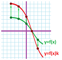
Next, what about the formula for the new function after the plane has been stretched? Suppose a point $(x,y)$ lies on the graph of $f$, then $f(x)=y$. After the stretch, the point $(x,ky)$ lies on the graph of the new function $g$, hence $g(x)=ky=kf(x)$.

Such a stretch can be carried out point by point:

Rule 5 (vertical stretch): If the graph of $y = g(x)$ is the graph of $y = f(x)$ stretched vertically by a factor of $k > 0$, then $$g(x) = kf(x),$$ and vice versa.

What about horizontal stretch? This time, we grab it by the left and right edges of the rubber sheet and pull them apart in such a way that the $y$-axis doesn't move. For example, a stretch by a factor of $2$ is shown below:

Once again, we understand “stretched by a factor $k$” as “shrunk by a factor $1/k$”. This is a way describe a horizontal stretch ($k>0$): $$\newcommand{\ra}[1]{\!\!\!\!\!\xrightarrow{\quad#1\quad}\!\!\!\!\!} \newcommand{\da}[1]{\left\downarrow{\scriptstyle#1}\vphantom{\displaystyle\int_0^1}\right.} \begin{array}{ccc} (x,y)& \ra{ \text{ horizontal stretch by } k}& (x\cdot k,y). \end{array}$$

Next, what about the formula for the new function after the plane has been stretched, horizontally? Suppose a point $(x,y)$ lies on the graph of $f$, then $f(x)=y$. After the stretch, the point $(kx,k)$ lies on the graph of the new function $g$, hence $g(kx)=y=f(x)$. Therefore, $g(x)=f(x/k)$.

Such a stretch can be carried out point by point:

Rule 6 (horizontal stretch): If graph $y = g(x)$ is the graph of $y = f(x)$ stretched by the factor $k>0$ horizontally, then $$g(x) = f(x/k),$$ and vice versa.

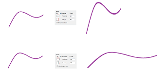
It is clear that the new function has a somewhat different shape of the graph than the old one.

Example. One can stretch and shrink with image processing software:

$\square$

Now the algorithmic interpretation of these operations. A vertical stretch, factor $3$: $$ \newcommand{\ra}[1]{\!\!\!\!\!\xrightarrow{\quad#1\quad}\!\!\!\!\!} \newcommand{\da}[1]{\left\downarrow{\scriptstyle#1}\vphantom{\displaystyle\int_0^1}\right.} % \begin{array}{ccccccccccccccc} x & \mapsto & \begin{array}{|c|}\hline\quad f \quad \\ \hline\end{array} & \mapsto & u & \mapsto & \begin{array}{|c|}\hline\quad 3u \quad \\ \hline\end{array} & \mapsto & y \end{array}$$ A horizontal stretch, factor $2$: $$ \newcommand{\ra}[1]{\!\!\!\!\!\xrightarrow{\quad#1\quad}\!\!\!\!\!} \newcommand{\da}[1]{\left\downarrow{\scriptstyle#1}\vphantom{\displaystyle\int_0^1}\right.} % \begin{array}{ccccccccccccccc} x & \mapsto & \begin{array}{|c|}\hline\quad x/2 \quad \\ \hline\end{array} & \mapsto & u & \mapsto & \begin{array}{|c|}\hline\quad f \quad \\ \hline\end{array} & \mapsto & y \end{array}$$

These stretches can also be described a uniform deformation away from the $y$-axis and a uniform deformation away from the $y$-axis respectively. That is why the former only changes the $x$-coordinates of the points and the latter only the $y$-coordinates.

Example. It seems that vertical stretching is somehow equivalent to horizontal shrinking. Consider $$ f(x) = x. $$ Stretched by a factor $2$ vertically it becomes: $$ g(x) = 2 x. $$ Shrunk by a factor $2$ horizontally it becomes: $$ h(x) = x/\tfrac{1}{2}=2x. $$ It is the same function.

However, if we do the same to $f(x)=x^2$, we discover that $$2 x^{2} \ne (2 x )^{2}!$$

Let's try the horizontal stretch by $\sqrt{2}$. Then $$g(x) = (\sqrt{2} x )^{2}.$$ Now there is a match: $$(\sqrt{2} x)^{2} =2 x^{2}.$$ $\square$

Exercise. What happens to the $x$- and $y$-intercepts of a function under vertical and horizontal stretches?

Exercise. What happens to the domain and the range of a function under vertical and horizontal stretches?

Exercise. Show that any quadratic function $f(x)=ax^2+bx+c$ can be represented as $f(x)=a(x-h)^2+k$ for some numbers $h,k$ and consequently its graph can be acquired from $y=x^2$ via the above transformations.

Exercise. (a) How do these transformations affect the monotonicity of a function? (b) Investigate the monotonicity of quadratic functions.

We can see that the transformations of the plane are functions of their own and a new function is produced from a function $f$ by linking one of them to the diagrams of $f$. We call this linking compositions.

Compositions

Compositions of functions can be illustrated as flowcharts:

$$ \newcommand{\ra}[1]{\!\!\!\!\!\xrightarrow{\quad#1\quad}\!\!\!\!\!} \newcommand{\da}[1]{\left\downarrow{\scriptstyle#1}\vphantom{\displaystyle\int_0^1}\right.} % \begin{array}{ccccccccccccccc} x & \mapsto & \begin{array}{|c|}\hline\quad x+3 \quad \\ \hline\end{array} & \mapsto & y & \mapsto & \begin{array}{|c|}\hline\quad y\cdot 2 \quad \\ \hline\end{array} & \mapsto & z & \mapsto & \begin{array}{|c|}\hline\quad z^2 \quad \\ \hline\end{array} & \mapsto & u \end{array}$$ Note how the names of the variables match so that we can proceed to the next step. An algebraic representation of the diagram is below: $$y=x+3,\quad z=y\cdot 2,\quad u=z^2.$$ It is also possible but not required to name the functions, say $f,g,h$. Then we have: $$y=f(x)=x+3,\quad z=g(y)=y\cdot 2,\quad u=h(z)=z^2.$$

As we see, with the variables properly named, composition is substitution, Indeed,

• we substitute $z=g(y)=y\cdot 2$ into $u=h(z)=z^2$, which results in the following:

$$u=h(z)=h(g(y)), \quad u=z^2=(y\cdot 2)^2.$$

• we substitute $y=f(x)=x+3$ into $z=g(y)=y\cdot 2$, which results in the following:

$$z=g(y)=g(f(x)), \quad z=y\cdot 2=(x+3)\cdot 2.$$

In general, we represent a function $f$ diagrammatically as a black box that processes the input and produces the output: $$ \newcommand{\ra}[1]{\!\!\!\!\!\xrightarrow{\quad#1\quad}\!\!\!\!\!} \newcommand{\da}[1]{\left\downarrow{\scriptstyle#1}\vphantom{\displaystyle\int_0^1}\right.} % \begin{array}{ccccccccccccccc} \text{input} & & \text{function} & & \text{output} \\ x & \mapsto & \begin{array}{|c|}\hline\quad f \quad \\ \hline\end{array} & \mapsto & y \end{array} $$

Now, what if we have another function $g$: $$ \newcommand{\ra}[1]{\!\!\!\!\!\xrightarrow{\quad#1\quad}\!\!\!\!\!} \newcommand{\da}[1]{\left\downarrow{\scriptstyle#1}\vphantom{\displaystyle\int_0^1}\right.} % \begin{array}{ccccccccccccccc} \text{input} & & \text{function} & & \text{output} \\ x & \mapsto & \begin{array}{|c|}\hline\quad g \quad \\ \hline\end{array} & \mapsto & y \end{array} $$ How do we represent their composition $g \circ f$? To represent it as a single function, we need to “wire” their diagrams together consecutively: $$ \newcommand{\ra}[1]{\!\!\!\!\!\xrightarrow{\quad#1\quad}\!\!\!\!\!} \newcommand{\da}[1]{\left\downarrow{\scriptstyle#1}\vphantom{\displaystyle\int_0^1}\right.} % \begin{array}{ccccccccccccccc} x & \mapsto & \begin{array}{|c|}\hline\quad f \quad \\ \hline\end{array} & \mapsto & y& \ne&x & \mapsto & \begin{array}{|c|}\hline\quad g \quad \\ \hline\end{array} & \mapsto & y \end{array}$$ But its only possible when the output of $f$ coincides with the input of $g$. We have to rename the variables of $g$. Then we have what we want: $$ \begin{array}{ccccccccccccccc} & x & \mapsto & \begin{array}{|c|}\hline\quad f \quad \\ \hline\end{array} & \mapsto & y & \mapsto & \begin{array}{|c|}\hline\quad g \quad \\ \hline\end{array} & \mapsto & z \end{array}$$ Then we have a diagram of a new function: $$ \begin{array}{ccccccccccccccc} g\circ f:& x & \mapsto & \begin{array}{|c|}\hline x & \mapsto & \begin{array}{|c|}\hline\quad f \quad \\ \hline\end{array} & \mapsto & y & \mapsto & \begin{array}{|c|}\hline\quad g \quad \\ \hline\end{array} & \mapsto & z \\ \hline\end{array} & \mapsto & z \end{array}$$ It's just another black box: $$ \begin{array}{ccccccccccccccc} & x & \mapsto & \begin{array}{|c|}\hline \quad g\circ f \quad \\ \hline\end{array} & \mapsto & z \end{array}$$

Example. The composition of $$g(x)=x^2 \text{ and } f(x)=x+2$$ is in fact the composition of $$z=g(y)=y^2 \text{ and } y=f(x)=x+2,$$ after re-naming. Then we just substitute the latter into the former: $$(g\circ f)(x)=g(f(x))=g(x+2)=(x+2)^2.$$ $\square$

Example. Represent $z = h(x) = \sqrt[3]{x^{2} + 1 }$ as the composition of two functions: $$ x \mapsto y=x^{2} + 1 \mapsto z=\sqrt[3]{y} . $$ To confirm, substitute back... $\square$

Example. Suppose a car is driven at $60$ m/h). Suppose we also know the the car uses $30$ m/gal, while the cost per gallon is $\$ 5$. Represent the expense as a function of time.

Analysis: $$ \text{time (hours)} \xrightarrow{\ 60\text{ m/h }\ } \text{distance (miles)}\xrightarrow{\ 30\text{ m/gal }\ } \text{gas used (gal)} \xrightarrow{\ \$ 5/ \text{ gal }}\text{expense } (\$) $$ We represent the procedure as a composition: $$ t \mapsto \underset{f}{60 t} \mapsto d \mapsto w \underset{k}{\frac{d}{30}} \mapsto g \mapsto \underset{h}{5 g} \mapsto e, $$ or, algebraically: $$ d = f(t) = 60t, \; g = k(d) = \frac{d}{30} \; e = h(g) = 5g. $$ Substitute: $$\begin{aligned}g = k(d) & = k(f(t)) \\ e = h(g) & = h(k(d)) \\ & = h(k(f(t))) \end{aligned}$$ We read from right to left though: $f(t)$ is not $(t)f$. $\square$

Example. $f(x) = x^{2}$ and $g(x) = \cos x$. To find $f(g(x))$, replace (substitute) $x$ in $f$ with $(\cos x )$, always with parentheses: $$ x^{2} \Longrightarrow ( \cos x )^{2}, $$ or $\cos^{2} x$. To find $g(f(x))$, replace $x$ in $g$ with $(x^{2})$: $$ \cos x \rightarrow \cos (x^{2}). $$ $\square$

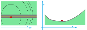
Example. Suppose a car is driven through a mountain terrain. The location, as seen on a map, is known and so is the altitude for each location.

We set up two functions, for location and altitude, and their composition is what we are interested in:

The second function is literally the profile of the road.

We already know that if the location, $f$, depends on time continuously and the altitude, $g$, depends continuously on location, then the altitude depends on time continuously as well, $g\circ f$.

Suppose

• $t$ is time measured in $\text{hr}$,
• $x=f(t)$ is the location of the car as a function of time -- measured in $\text{mi}$,
• $y=g(x)$ is the altitude of the road as a function of (horizontal) location -- measured in $\text{ft}$, and
• $y=h(t)=g(f(t))$ is the altitude of the road as a function of time -- measured in $\text{ft}$.

$\square$

This is the familiar way to evaluate a function: $$f(x)=x^2-x\ \Longrightarrow\ f(3)=3^2-3.$$ Let's consider an alternative notation for substitution: $$f(x)=x^2-x\ \Longrightarrow\ f(3)=x^2-x\Bigg|_{x=3}=3^2-3.$$ This notation also applies to compositions. For example,

• we substitute $z=g(y)=y\cdot 2$ into $u=h(z)=z^2$, which results in the following:

$$u=z^2\Bigg|_{z=y\cdot 2}=(y\cdot 2)^2.$$

• we substitute $y=f(x)=x+3$ into $z=g(y)=y\cdot 2$, which results in the following:

$$z=y\cdot 2\Bigg|_{y=x+3}=(x+3)\cdot 2.$$

Inverses

Historically, some new algebraic operations may have appeared as repeated “old” operations; for example, repeated addition: $$ 2 + 2 + 2 = 2 \cdot 3, $$ leads to a new operation: multiplication. Meanwhile, repeated multiplication: $$ 2 \cdot 2 \cdot 2 \cdot 2 = 2^{4}. $$ leads to a new operation: exponent.

But what about subtraction and division? How do they appear? It's different.

Example. Suppose I know how to add. Problem: I have $\$5$, how much do I add to have $\$ 12$? Answer: $\$ 7$. How do I know? Algebra: solve $$ 5 + x = 12. $$ This equation leads to a new operation, subtraction: $x = 12 - 5$. Subtraction is the “inverse” of addition. $\square$

Example. Suppose now I know to multiply. Problem: I have a few $2$-by-$4$s and I need a table $20$ inches wide. How many do I need? Answer: $5$. How do I know? Algebra: solve $$ 4x = 20 .$$ This equation leads to a new operation, division: $x = \frac{20}{4}$. Division is the “inverse” of multiplication. $\square$

Example. I need a square table of area 25 square feet. What is the width of the table? Algebra: Solve $$ x \cdot x = 25 \Longrightarrow x^{2} = 25 \Longrightarrow x = \sqrt{25} .$$ Thus, we have a new operation: square root. It is the “inverse” of square. $\square$

Example. What about $\sqrt[3]{}$? What is the side of a box given a volume of $8$ cubic feet? Solve $$ x^{3} = 8 \Longrightarrow x = \sqrt[3]{8}. $$ $\square$

Thus, solving equations requires us to undo some operations present in the equation: $$\begin{array}{rl} x+2=5& \Longrightarrow & (x+2)-2=5-2& \Longrightarrow &x=3;\\ 3x=6&\Longrightarrow & (3x)/3=6/3&\Longrightarrow &x=2;\\ x^2=4&\Longrightarrow & \sqrt{x^2}=\sqrt{4}& \Longrightarrow &x=\pm 2. \end{array}$$

But these are functions! And some functions undo the effect of others:

• the addition of $2$ is undone by the subtraction of $2$, and vice versa;
• the multiplication by $3$ is undone by the division by $3$, and vice versa;
• the second power is undone by the square root (for $x\ge 0$), and vice versa.

Each of these undoes the effect of its counterpart under substitution:

• substituting $y=x+2$ into $x=y-2$ gives us $x=x$;
• substituting $y=3x$ into $x=\frac{1}{3}y$ gives us $x=x$;
• substituting $y=x^2$ into $x=\sqrt{y}$ gives us $x=x$, for $x,y\ge 0$.

And vice versa!

• substituting $x=y-2$ into $y=x+2$ gives us $y=y$;
• substituting $x=\frac{1}{3}y$ into $y=3x$ gives us $y=y$;
• substituting $x=\sqrt{y}$ into $y=x^2$ gives us $y=y$, for $x,y\ge 0$.

More precisely, they undo each other under composition, as follows.

Definition. Two functions $y=f(x)$ and $x=g(y)$ are called inverse of each other when for all $x$ in the domain of $f$ and for all $y$ in the domain of $g$, we have for all $x$ and $y$: $$g(f(x))=x \text{ and } f(g(y))=y.$$

The inverse of function $f$ is denoted by $x=f^{-1}(y)$,

Thus, we have three pairs of inverse functions: $$\begin{array}{rl} f(x)=x+2& \text{ vs. }& f^{-1}(y)=y-2,\\ f(x)=3x&\text{ vs. }& f^{-1}(y)=\frac{1}{3}y,\\ f(x)=x^2&\text{ vs. }& f^{-1}(y)=\sqrt{y} \quad\text{ for }x,y\ge 0. \end{array}$$

Note: here “$f$” is the name of the old function and “$f^{-1}$” is the name of the new function.

Example. Suppose the function is given numerically, by a table: $$\begin{array}{l|l} x&y=f(x)\\ \hline 0&1\\ 1&10\\ 2&-1\\ ... \end{array}$$ Then the table of the inverse is obtained by interchanging the columns: $$\begin{array}{l|l} y&x=f^{-1}(y)\\ \hline 1&0\\ 10&1\\ -1&2\\ ... \end{array}$$ A question then arises, does this table represent a function? To answer this question, we would have to check every row of the table to make sure that we don't have something like this: $$\begin{array}{l|l} y&x=f^{-1}(y)\\ \hline ...\\ 1000&1\\ ...\\ 1000&2\\ ... \end{array}$$ $\square$

These are the conditions of the definition written via the compositions of the functions: $$(g\circ f)(x)=x \text{ and } (f\circ g)(y)=y,$$ or $$g(y)\Bigg|_{y=f(x)}=x \text{ and } f(x)\Bigg|_{x=g(y)}=y.$$ And that is the diagram representation: $$ \newcommand{\ra}[1]{\!\!\!\!\!\xrightarrow{\quad#1\quad}\!\!\!\!\!} \newcommand{\da}[1]{\left\downarrow{\scriptstyle#1}\vphantom{\displaystyle\int_0^1}\right.} % \begin{array}{ccccccccccccccc} x & \mapsto & \begin{array}{|c|}\hline\quad f \quad \\ \hline\end{array} & \mapsto & y & \mapsto & \begin{array}{|c|}\hline\quad f^{-1} \quad \\ \hline\end{array} & \mapsto & x \text{, same! } \end{array}$$ $$ \newcommand{\ra}[1]{\!\!\!\!\!\xrightarrow{\quad#1\quad}\!\!\!\!\!} \newcommand{\da}[1]{\left\downarrow{\scriptstyle#1}\vphantom{\displaystyle\int_0^1}\right.} % \begin{array}{ccccccccccccccc} y & \mapsto & \begin{array}{|c|}\hline\quad f^{-1} \quad \\ \hline\end{array} & \mapsto & x & \mapsto & \begin{array}{|c|}\hline\quad f \quad \\ \hline\end{array} & \mapsto & y \text{, same! } \end{array}$$

Example. This is a familiar pair of inverse functions: $$ \newcommand{\ra}[1]{\!\!\!\!\!\xrightarrow{\quad#1\quad}\!\!\!\!\!} \newcommand{\da}[1]{\left\downarrow{\scriptstyle#1}\vphantom{\displaystyle\int_0^1}\right.} % \begin{array}{ccccccccccccccc} x & \mapsto & \begin{array}{|c|}\hline\quad \text{ square } \quad \\ \hline\end{array} & \mapsto & y & \mapsto & \begin{array}{|c|}\hline\quad \text{ square root} \quad \\ \hline\end{array} & \mapsto & x \text{, same? } \end{array}$$ No, the diagram fails if we plug in $x=-2$: $$ \newcommand{\ra}[1]{\!\!\!\!\!\xrightarrow{\quad#1\quad}\!\!\!\!\!} \newcommand{\da}[1]{\left\downarrow{\scriptstyle#1}\vphantom{\displaystyle\int_0^1}\right.} % \begin{array}{ccccccccccccccc} -2 & \mapsto & \begin{array}{|c|}\hline\quad \text{ square } \quad \\ \hline\end{array} & \mapsto & 4 & \mapsto & \begin{array}{|c|}\hline\quad \text{ square root} \quad \\ \hline\end{array} & \mapsto & 2 \text{, not the same! } \end{array}$$ $\square$

Conclusion: Not all functions have inverses.

However, we can make it work by restricting the domain of the function.

Example. Old function: $y = x^{2}$, with the domain assumed to be $(-\infty, \infty)$. It simply doesn't have the inverse!

New function: $y = x^{2}$, with the domain chosen to be $[0, \infty )$. Then it works: this function has the inverse as we know.

What was the problem? We know that $$ 2^{2} = 4. $$ But we eliminated this possibility $$ (-2)^{2} = 4. $$ The conflict is visible in this diagram: $$f:\begin{array}{lll} 2\\ &\searrow\\ &&4\\ &\nearrow\\ -2 \end{array}\qquad\qquad f^{-1}:\begin{array}{lll} 2\\ &\nwarrow\\ &&4\\ &\swarrow\\ -2 \end{array} $$ The “inverse” is a relation but not not a function as there are two outputs for the same input. $\square$

What we need to require from a function is that two different inputs cannot produce the same output.

Definition. A function $y = f(x)$ is called a one-to-one if $$ f(x_{1}) \neq f(x_{2}) $$ unless $x_{1} = x_{2}$. Such a function is also called invertible.

In other words, there is only one $x$ for each $y$.

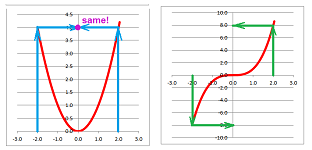
Example. $f(x)=x^{2}$ is not one-to one but $g(x)=x^{3}$ is. It is easy to see the problem with the former: $1^2=(-1)^2=1$.

$\square$

What is the difference? Two points on the graph have the same height above the $x$-axis!

Theorem (Horizontal Line Test). A function is one-to-one if and only if every horizontal line has at most one intersection with its graph.

Theorem. All monotonic functions are one-to-one.

Thinking geometrically, the graph of an increasing function can't come back and cross a horizontal line for the second time:

Now, algebraically, this is the definition: $$ f\nearrow \textrm{ when: } \underbrace{x_{1} < x_{2}}_{\textrm{two different inputs}} \Longrightarrow \underbrace{f(x_{1}) < f(x_{2})}_{\textrm{two different outputs}} .$$ Hence $f$ is one-to-one.

Theorem. The odd powers are one-to-one. The even powers aren't one-to-one. The even powers with domains reduced to $[0,\infty)$ or $(-\infty,0]$ are one-to-one.

The reason is that the former are monotonic and the latter aren't.

Next, what is the relation between the graph of a function and the graph of its inverse?

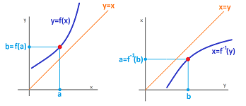
In other words, what do we do with the graph of $f$ to get the graph $f^{-1}$? Technically, we don't need to do anything. Sounds strange, but consider this. The graph of $f$ illustrates how $y$ depends on $x$... as well as how $x$ depends on $y$. But the latter is what determines $f^{-1}$! So, there is no need for a new graph -- the graph of $f^{-1}$ is the graph of $f$. The only problem is that the $x$- and $y$-axes point in the wrong directions. How can we fix that?

Example. Replacing $f$ with its inverse $f^{-1}$, $$\begin{array}{l|l} x&y=f(x)\\ \hline 0&1\\ 1&10\\ 2&-1\\ ... \end{array}\quad \leadsto \quad \begin{array}{l|l} y&x=f^{-1}(y)\\ \hline 1&0\\ 10&1\\ -1&2\\ ... \end{array}$$ replaces every point $(x,y)$ in the $xy$-plane with a point $(y,x)$ in the $yx$-plane:

$\square$

We realize that this is a reflection of the plane with respect to the diagonal line $y=x$.

Such a transformation of the plane can be accomplished with image processing software by first rotating the image clockwise $90$ degrees and then flipping it vertically:

We take the graph of the former function and flip this piece of paper so that the $x$-axis and the $y$-axis are interchanged. Then we get the graph of the latter (and vice versa):

The shapes of the graphs are the same!

Example. Suppose a function is given only by its graph. Find the graph of the inverse $x = f^{-1}(y)$.

Start with choosing a few points on the graph, especially with ones easy to find counterparts (points on the axes, points on the diagonal, etc.). Plot their counterpart points: from the point go perpendicular to the diagonal ($45$ degrees) and then measure the same distance on the other side. Then draw a curve that connects these new points. $\square$

Example. Suppose a function is given only by its formula. Find the formula of the inverse $x = f^{-1}(y)$. For example, let $$f(x)=x^3-3.$$ We simply rewrite $$y=x^3-3,$$ and then solve for $x$: $$x=\sqrt[3]{y+3}.$$ Thus the answer is: $$f^{-1}(y)=\sqrt[3]{y+3}.$$ $\square$

While solving the equation $y=f(x)$ for $x$, we are watching out for multiple answers, such as $$y=x^2\ \Longrightarrow\ x=\pm\sqrt{y},$$ or $$y=|x|\ \Longrightarrow\ x=\pm y.$$

We then recognize that these functions are not one-to-one.

exercise. Prove that a one-to-one function can have only one inverse.

Algebraic functions

Algebraic functions are the ones “with roots”...

The roots appear as the inverses of the power functions, i.e., $x^n$ for a positive integer $n$:

• $y=\sqrt{x}$ is the inverse of $x=y^2,\ y\ge 0$;
• $y=\sqrt[3]{x}$ is the inverse of $x=y^3$;
• $y=\sqrt[4]{x}$ is the inverse of $x=y^4,\ y\ge 0$;
• ...
• $y=\sqrt[n]{x}$ is the inverse of $x=y^n$ with domain $y\ge 0$ when $n>1$ is even.

Example. Find the domain to the function $$ \sqrt{ x - \sqrt{x}}. $$ Whatever is inside the square root can't be negative. So, we need to find all $x$ for which

• first, $x \geq 0$, i.e., $x$ is positive; and
• second, $x - \sqrt{x} \geq 0$.

Solve it: $$ \begin{aligned}x & \geq \sqrt{x} \\ x^{2} & \geq x \\ x & \geq 1 \end{aligned}$$ The domain is $$D = [1, \infty). $$ $\square$

Example. Given $$ y = \sqrt{u} + \sqrt{4 - u},$$ find the domain, i.e., find all $u$'s for which the formula makes sense.

Make sure that $\sqrt{\, ?\,}$ makes sense, i.e., what's inside cannot be negative.

• $\sqrt{u}\ \Longrightarrow\ u \geq 0$;
• $\sqrt{4 - u} \ \Longrightarrow\ 4 - u\ge 0$, solve: $ u \leq 4$.

Each $u$ in the domain must satisfy both inequalities, $$u \geq 0 \text{ AND } u \leq 4.$$ Hence, the domain is: $$ D = [0,4]. $$ $\square$

Once the roots are understood, a new notation is introduced:

• $x^{1/2}=\sqrt{x},$
• $x^{1/3}=\sqrt[3]{x},$
• $x^{1/4}=\sqrt[4]{x},$
• ...
• $x^{1/n}=\sqrt[n]{x}$ for any positive integer $n$.

Furthermore, we can have notation any rational power, $x^p$. Indeed, if $p=m/n$, where $m,n$ are integers with $n\ne 0$, then we define: $$x^{m/n}=\sqrt[n]{x^m}.$$

Trigonometric functions

These three will suffice $99\%$ of the time: $$ \sin x,\ \cos x,\ \tan x = \frac{\sin x}{\cos x}. $$

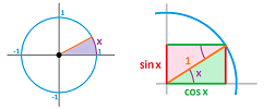
Suppose a real number $x$ is given. We construct a line segment of length $1$ on the plane with angle $x$ from the $x$-axis. Then

• $\cos x$ is the projection of the segment on the horizontal line,
• $\sin x$ is the projection of the segment on the vertical line.

It is as though $\cos x$ is the length of the shadow of the stick on the ground when the sun is above and $\sin x$ is the length of its shadow on the wall at sunset...

The domain for $\sin$ and $\cos$ are all real numbers.

These functions are periodic, with period $2\pi$: $$ \begin{aligned} \sin( x + 2 \pi ) & = \sin x, \\ \cos(x + 2\pi) & = \cos x, \\ \end{aligned}$$ for all $x$.

Neither function is one-to-one. What we did with $y=x^2$ vs. $x=\sqrt{x}$ and will repeat here is:

• restrict the domain of the function to be able to define its inverse.

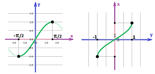
We choose the branch of $\sin$ over $-\pi/2 \le x \le \pi/2$. Thus, we have a pair of inverse functions, the sine (restricted) and the arcsine: $$y=\sin x,\ x\in [-\pi/2,\pi/2], \text{ and } x=\sin^{-1}y,\ y\in [-1,1].$$

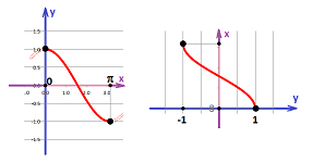
The graphs are of course the same with just $x$ and $y$ interchanged. Similarly, we choose the branch of $\cos$ over $0 \le x \le \pi$. Thus, we have a pair of inverse functions, the cosine (restricted) and the arccosine: $$y=\cos x,\ x\in [0,\pi], \text{ and } x=\cos^{-1}y,\ y\in [-1,1].$$

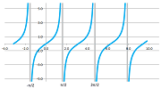
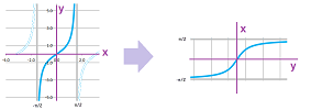
What about the tangent?

To find the domain of a fraction, such as $$\tan x =\frac{\sin x}{\cos x},$$ set the denominator equal to $0$ and solve. Find all $x$'s: $$\begin{aligned} \cos x & = 0 \ \Longrightarrow\\ x & = ..., \frac{\pi}{2}, \frac{3\pi}{2}, \frac{5\pi}{2}, ... \end{aligned}$$ Then we should choose the branch of $\tan$ over $-\pi/2< x< \pi/2$. Then, we again have a pair of inverse functions, the tangent (restricted) and the arctangent: $$y=\tan x,\ x\in (-\pi/2,\pi/2), \text{ and } x=\tan^{-1}y,\ y\in (-\infty,+\infty).$$

Exponential functions

Where does it come from? Remember this simple algebra:

• Addition: $2 + 2 + 2 = 2 \cdot 3 \leadsto$ multiplication.

That's how multiplication was “invented” -- as repeated addition. What about repeated multiplication?

• Multiplication: $2 \cdot 2 \cdot 2 = 2^{3} \leadsto$ exponent.

Here we have: $$\begin{array}{rl} &\text{exponent}\\ &\downarrow\\ &\small{3}\\ 2\\ \uparrow\\ \text{base} \end{array}$$

Now the algebraic properties of the exponent...

Multiplication property: $$a^{m} \cdot a^{n} = a^{m + n}$$

As in: $$\begin{aligned} 2^{3} \cdot 2^{2} & = (2 \cdot 2 \cdot 2) \cdot (2 \cdot 2 ) \\ & = 2 \cdot 2 \cdot 2 \cdot 2 \cdot 2& = 2^{5}. \end{aligned}$$

Division property: $$\dfrac{a^{m}}{a^{n}} = a^{m-n}$$

Just canceling, as in: $$\frac{2^{4}}{2^{2}} = \frac{2 \cdot 2 \cdot 2 \cdot 2}{2 \cdot 2} = 2 \cdot 2 = 2^{2}. $$

Power property: $$(a^{m})^{n} = a^{mn} = (a^{n})^{m}.$$

As in: $$ \begin{aligned} (2^{3})^{2} & = 2^{3} \cdot 2^{3} \\ & = ( 2 \cdot 2 \cdot 2 ) ( 2 \cdot 2 \cdot 2 ) \\ & = 2^{6}. \end{aligned}$$

Distributive property: $$(ab)^{n} = a^{n} b^{n}.$$

Example. Bacteria double in number every day. Then, $$10 \text{ days: } 10 \cdot 2^{10} = 10.1024 = 10,240.$$ $\square$

Now the exponent as a function...

We would like to have a function defined for all $x$, i.e., domain = $(-\infty, \infty)$. So far, $a^{x}$ is defined only if $x$ is a positive integer (and $a>0$).

Let's try to fill in the blanks... What about $x = \frac{1}{2}$?

What is $$ 2^{\frac{1}{2}} = ? $$ As before, we interpret it as $\sqrt{2}$, which is a number $u$ such that $$ u^{2} = 2. $$ Similarly for $x = \dfrac{1}{3}$, we have $$ 2^{\frac{1}{3}} = \sqrt[3]{2}. $$

We get more and more but there are still gaps:

Example. Consider what happens to a $\$1000$ deposit with $10\%$ annual interest, compounded yearly: $$ \begin{aligned} \$ 1000, 1000 \cdot 1.10 & = 1000 + 10\% \textrm { of } 1000 \\ \textrm{begin, after 1 year } & = \textrm{ principal } + \textrm{ interest} \\ & = 1000 + 1000 \cdot .10 \\ & = 1000(1 + 0.1 ) \\ & = 1000 \cdot 1.1 . \end{aligned}$$ After $x$ years: $1000\cdot 1.1^{x}$, where $x$ is a positive integer. $\square$

More generally, $$ 2^{\frac{p}{q}} = \sqrt[q]{2^{p}} $$ Here $\dfrac{p}{q}$ is a rational number, i.e., $p, q$ are integers with $p \neq 0$.

This is our interpretation of rational exponents.

Even though the points seem to form a curve, there are still “invisible” gaps! Indeed, irrational $x$'s are missing: $$x= \sqrt{2},\ \sqrt{3},\ \pi .$$ What happens is, roughly, that we define the function for irrational exponents by “approximating” them with rational numbers. It is called the “limit” to be discussed later.

Furthermore, there is an exponential function for each real $a > 0$.

we nest consider the properties of the exponential function.

Let's collect some facts about the graph of this function:

• the domain is $(-\infty,+\infty)$;
• the range is $(0, \infty)$;
• the $y$-intercept is $(0, 1)$;
• there are no $x$-intercepts.

Indeed term “exponential growth” makes sense: the graph of $2 ^{x}$ is rising. The general result is the following.

Theorem (Monotonicity of Exponent). $$ \begin{aligned} a^{x} & \textrm{ is increasing if } a > 1, \\ a^{x} & \textrm{ is decreasing if } a < 1, \end{aligned} $$ for $a > 0$ and $a \neq 1$.

Proof. Suppose $x_1$ and $x_2$ are integers and $x_1<x_2$. Then the following is derived from the rules of inequalities: \begin{array}{lll} a>1&\Longrightarrow& a^{x_1}>a^{x_2},\\ 0<a<1&\Longrightarrow& a^{x_1}<a^{x_2}. \end{array} The non-integer exponents will be addressed later. $\blacksquare$

Example. A familiar exercise is to plot $2^{3x}$. Once we have, point by point, we realize that it looks very similar to the exponential functions we have seen:

A bit of algebra reveals the connection: $$2^{3x} = (2^{3})^{x} = 8^{x}.$$ It is an exponential function (base $8$). So, turns out $8^{x}$ is $2^{x}$ shrunk horizontally by a factor of $3$. $\square$

Example. It is even easier to recognize $2^{-x}$ as a exponential function: $$2^{-x}= \frac{1}{2^{x}}= \left(\frac{1}{2}\right)^{x}.$$

This is an exponential function (base $1/2$). So, turns out $2^{-x}$ is $2^{x}$ flipped about the $y$-axis. $\square$

Lesson: We can get all exponential functions by stretching and flipping one of them.

So, just as we need only one quadratic polynomial, $x^2$, we only need one exponential function!

Which one? It is $e^{x}$, the natural base exponent. It has a special property: it crosses the $y$-axis at $45$ degrees:

Example. Population growth: $50$ babies per $10,000$ of population. $$ \frac{50}{10000} = 0.005. $$ Therefore, $$ 1,000,000 \cdot 1.005^{x}. $$ What is the multiple? It's the base of exponent. $\square$

Logarithm

Example. Bacteria doubles every day. How long does it take to go $8$-fold? Start with equation and solve $$ 2^{x} = 8, $$ where $x$ is the time in days. Then $$ x = \log_{2} 8. $$ The logarithm base $2$ is the inverse of the exponential function base $2$. $\square$

Example. Solve the following for $x$. $$ y = 2^{x-5} = 3. $$ To “kill” the exponent and get to $x$, apply its inverse -- to both sides of the equation: $\log_{2} y$ (same base!). Then $$ \log_{2} (2^{x - 5}) = \log_{2} (3) $$ Use the property of the inverse and “cancel”: $$ \begin{aligned} x - 5 & = \log_{2} 3 \\ x & = \log_{2} 3 + 5. \end{aligned} $$ If $a^{x} = y$ then $x = \log _{a} y$, and vice versa. Recall also this: if $$ a \cdot a \cdot ... a = ax, $$ $x$ times, then $$ \log_{a} \underbrace{a \cdot a \cdot ... a}_{x \textrm{ times}} = x. $$ $\square$

Example. $$ \begin{alignat}{2} \log_{10} 100 & = 2 & \quad \log_{5} 125 = 3 \\ \log_{2} \frac{1}{2} & = -1 & \quad \log_{2}\sqrt{2} &= \frac{1}{2}. \end{alignat} $$ $\square$

Definition. The logarithm base $a$ of $y$, $\log_{a} y$, is the power to which you have to raise $a$ to get $y$.

Consider: $$ \begin{aligned} \log_{a} \underbrace{ ( a^{m}\cdot a^{n} ) }_{\textrm{multiplication}} & = \log_{a} (a^{m + n}) \\ & = m + n \\ & = \log_{a} a^{m} \underset{\textrm{addition}}{+} \log_{a} a^{n} \\ \Longrightarrow \log_{a} (a^{m}\cdot a^{n}) & = \log_{a} a^{m} + \log_{a} a^{n}. \end{aligned} $$

Properties of logarithm

1. $$ \log_{a}(xy) = \log_{a} x + \log_{a} y ;$$
2. $$ \log_{a} \left(\frac{x}{y}\right) = \log_{a} x - \log_{a} y; $$
3. $$ \log_{a} (x^{y}) = y \log_{a} x .$$

Proof. Given $x = a^{n}$, compute: $$ \begin{aligned} \log_{a} (a^{n})^{y} & = \log_{a} a^{ny} \\ & = yn \\ & = y \log_{a} x. \end{aligned}$$ $\blacksquare$

Thus, each property of $ \log $ corresponds to a property of $\exp$.

Example. Find a representation $y=Ca^{x}$ for this graph:

Pick two points on the graph and use them to write two equations for $f(x) = C a^{x}$:

• $(0, 2)$ on the graph $\Rightarrow x = 0,\ y = 2 \Rightarrow Ca^{0} = 2 \Rightarrow C = 2 $;
• $(2, .25)$ on the graph $\Rightarrow x = 2,\ y = .25 \Rightarrow 2a^{2} = .25 $

$\square$

We can solve a variety of problems about the exponential function with the logarithm using the fact that the two, $\ln ?$ and $e^{?}$, always cancel each other: $$ \left.\begin{aligned} \ln e^{x} & = x \textrm{ for any } x \\ e^{\ln x} & = x \textrm{ for any } x>0 \end{aligned} \right\} \qquad \textrm{ cancellation property } $$

Now about the logarithm as a function... We simply use what we know about the exponent and what we know about inverses:

• the domain of $y=\log_a x$ is $(0,\infty)$,
• the range of $y=\log_a x$ is $(-\infty,\infty)$,
• $y=\log_a x$ is increasing when $a>1$ and decreasing when $0<a<1$.

Example. City loses $7\%$ of population every year - exponential decline: $$\overbrace{( \underbrace{\underbrace{(1,000 \cdot 0.93 )}_{\textrm{after 1 year}} \cdot 0.93}_{\textrm{after 2 years}} ) \cdot 0.93}^{\textrm{after 3 years}}.$$ Here the multiple is $< 1$, hence it is decreasing.

$\square$

Example. Find the inverse of $$y = \frac{e^{x}}{1 + 2e^{x}}.$$ Plan: solve the equation for $x$ while checking that it is one-to-one: $$ \begin{aligned} y ( 1 + 2e^{x}) & = e^{x} \\ y + y2e^{x} & = e^{x} \\ 2ye^{x} - e^{x} & = -y \\ (2y - 1 ) e^{x} & = - y \\ \Longrightarrow e^{x} & = -\frac{y}{2y - 1 } \end{aligned}$$ Apply the inverse, which is $\ln$, to both sides of the equation: $$ \underbrace{\ln e^{x}}_{x} = \ln\left(-\frac{y}{2y - 1}\right) \Longrightarrow\ x = \ln\left(-\frac{y}{2y - 1}\right) $$ To find the domain, solve: $$ \left. \begin{aligned} 2y - 1 & \neq 0 \\ -\frac{y}{2y - 1} & > 0 \end{aligned} \right\} \Longrightarrow\ D=(0,1/2).$$ $\square$

Example. Find the inverse of $$ f(x) = e^{x^{3}}.$$ (Note: This is not $(e^{x})^{3}$.)

Method: Equation $y = e^{x^{3}}$, solve for $x$. To get to $x$, we need to get rid of the exponent. To cancel it, apply its inverse to both sides.

For $e^{x}$ its $\ln$: $$ \begin{aligned} \ln y & = \ln e^{x^{3}} \\ \ln y & = x^{3} \end{aligned} $$ Apply the inverse to get to $x$ $$ \begin{aligned} \sqrt[3]{\ln y} & = \sqrt[3]{x^{3}} \\ & = x \end{aligned} $$ Answer: $ f^{-1}(y) = \sqrt[3]{\ln y} $. $\square$

Change of variables

The variables of the functions we are considering are quantities we meet in real life. These quantities often have multiple ways to be measured:

• length and distance: inches, miles, kilometers, light years;
• time: minutes, seconds, hours, years;
• weight: pounds, kilograms, karats;
• temperature: degrees of Celsius, of Fahrenheit,
• etc.

Example. Suppose we have a function $f$ that records the temperature -- in Fahrenheit -- as a function of time -- in minutes. Now, what $f$ should be replaced with if we want to records the temperature in Celsius as a function of time in seconds?

Let's name the variables:

• $s$ time in seconds;
• $m$ time in minutes;
• $F$ temperature in Fahrenheit;
• $C$ temperature in Celsius.

Then the original function is $$F=f(m),$$ and it is to be replaced with some $$C=g(s).$$

First, we need the conversion formulas for these units. First, the time. This is what we know: $$1 \text{ minute } = 60 \text{ seconds }.$$ However, this is not the formula to be used to convert $s$ to $m$ because these are the number of seconds and the number of minutes respectively. Instead, we have: $$m=s/60.$$

Second, the temperature: $$C=(F-32)/1.8.$$

These are the relations between the four quantities: $$g:\quad s \xrightarrow{\quad s/60 \quad} m \xrightarrow{\quad f\quad} F \xrightarrow{\quad (F-32)/1.8\quad} C.$$

The answer to our question is, we replace $f$ with $g$, the composition of the above functions: $$F=g(s)=(f(s/60)-32)/1.8.$$

Note that both of the conversion formulas are one-to-one functions! That's what guarantees that the conversions are unambiguous and reversible. More precisely, we say that these functions are invertible. Indeed, for the time: $$s=60m,$$ and for the temperature: $$F=1.8C+32.$$ $\square$

Mathematically, we see such a transition as a change of variables. Usually, it is done one at a time: either the dependent or the independent variable.

Note: We can interpret every composition as a change of variables.

Example. Suppose $t$ is time and $x$ is the location. Suppose also that function $g$ represents the change of units of length, such as from miles to kilometers: $$z=g(x)=1.6x.$$ Then, the change of the units will change very little; the coefficient, $m=1.6$, is the only adjustment necessary. If $f$ is the distance in miles, then $h$ is the distance in kilometers: $h(t)=1.6f(t)$. Thus, all the functions are replaced with their multiples. $\square$

Example. Degrees and radians: $$\pi \text{ radians } = 180 \text{ degrees }. $$ Therefore, the conversion of the number of degrees $d$ to the number of radians $r$ is: $$r=\frac{\pi}{180}d.$$ $\square$

Note that all of the conversion formulas have been provided by linear functions. Then

• a linear change of variables will cause the $x$-axis or the $y$-axis to shift, stretch, or flip.

Therefore, from what we know about transformations of functions' graphs,

• a linear change of variables will cause the graph of the function to shift, stretch, or flip.

Some nonlinear changes of variables are also known.

Example. The loudness of sound (the decibel) and the magnitude of earthquakes (the Richter scale) are measured on a logarithmic scale. This scale is based on orders of magnitude rather than a linear scale, i.e., the next mark on the scale corresponds to the previous mark multiplied by a given value, such as $10$:

Spreadsheet has an option to switch the scale in just a couple of clicks. For example, we can see how the graph of an exponential function becomes linear over a logarithmic scale (the $y$-axis):

$\square$

Review exercises

Example. Find two numbers whose difference is $100$ and the product is a minimum.

Step 1. Deconstruct:

• 1. two numbers, whose
• 2. difference is $100$, and
• 3. the product is a minimum.

Translate:

• 1. introduce the variables: $x$ is the first number, $y$ is the second number;
• 2. constraint: $x - y = 100;$
• 3. $P$ is their product: $P=xy$, minimize $P$.

This is a math problem now.

Step 2. Eliminate the extra variables to create a function of single variable to be maximized or minimized. The constraint, an equation connecting the variables, is: $$ x - y = 100.$$ Solve the equation for $y$: $$ y = x - 100 ,$$ and eliminate $y$ from $P$ by substitution: $$ P = xy = x(x - 100). $$

Step 3. Optimize this function: $$\begin{aligned} P(x) & = x^{2} - 100x \quad\Longrightarrow\\ P' &= 2x - 100 \\ &= 2x - 100\quad = 0. \end{aligned}$$ Solve for $x$: $$x = 50.$$

Step 4. Provide the answer using the original language of the problem: substitute $x$ into $y$, $$\begin{aligned} y &= x - 100 \\ &= 50 - 100 \\ &= -50. \end{aligned}$$ Answer: the two numbers are $50$ and $-50$. $\square$

Example. Plot the graph of the inverse of $y = f(x)$ shown below:

• Draw the diagonal $y = x$,
• pick a few points on the graph of $f$ (we choose four);
• plot a corresponding point for each of them:
  • on the line through point $A$ that is perpendicular to the diagonal (i.e., its slope is $45$ degrees down),
  • on the other side of the diagonal from $A$,
  • same distance from the diagonal as $A$;
• draw by hand a curve from point to point;
• verify the answer with drawing software.

$\square$

Example. Given functions $$f(x) = \dfrac{x}{1 + x},\ g(x) = \sin 2x,$$ find their compositions, $f \circ g$ and $g \circ f$, and their domains.

The composition $f \circ g$ is: $$ \newcommand{\ra}[1]{\!\!\!\!\!\xrightarrow{\quad#1\quad}\!\!\!\!\!} \newcommand{\da}[1]{\left\downarrow{\scriptstyle#1}\vphantom{\displaystyle\int_0^1}\right.} % \begin{array}{ccccccccccccccc} x & \mapsto & \begin{array}{|c|}\hline\quad g \quad \\ \hline\end{array} & \mapsto & y & \mapsto & \begin{array}{|c|}\hline\quad f \quad \\ \hline\end{array} & \mapsto & z \end{array}$$ This means that, in order to make their variables to match, we will have to rename them: $$ \newcommand{\ra}[1]{\!\!\!\!\!\xrightarrow{\quad#1\quad}\!\!\!\!\!} \newcommand{\da}[1]{\left\downarrow{\scriptstyle#1}\vphantom{\displaystyle\int_0^1}\right.} % \begin{array}{ccccccccccccccc} x & \mapsto & \begin{array}{|c|}\hline\quad \sin 2x \quad \\ \hline\end{array} & \mapsto & y & \mapsto & \begin{array}{|c|}\hline\quad \dfrac{y}{1 + y} \quad \\ \hline\end{array} & \mapsto & z \end{array}$$ Now we substitute $y = \sin 2x$ into $f(y)=\tfrac{y}{1 + y}$: $$\begin{aligned} (f \circ g )( x ) & = f(g(x)) = f(y) \\ & = \dfrac{y}{1 + y } \\ & = \dfrac{\sin 2x}{1 + \sin 2x} . \end{aligned} $$ To find the domain, solve: $1 + \sin 2x = 0$, as follows: $$ \begin{aligned} \sin 2x &= -1 \\ \Longrightarrow 2x & = -\frac{\pi}{2} + 2\pi k, \end{aligned} $$ where $k$ is any integer. Therefore, the domain is $$D= \{x:x\ne -\tfrac{\pi}{4} + \pi k,\ k=0,\pm 1,\pm 2,...\}. $$

Next we consider the composition $g \circ f$: $$ \newcommand{\ra}[1]{\!\!\!\!\!\xrightarrow{\quad#1\quad}\!\!\!\!\!} \newcommand{\da}[1]{\left\downarrow{\scriptstyle#1}\vphantom{\displaystyle\int_0^1}\right.} % \begin{array}{ccccccccccccccc} x & \mapsto & \begin{array}{|c|}\hline\quad f \quad \\ \hline\end{array} & \mapsto & y & \mapsto & \begin{array}{|c|}\hline\quad g \quad \\ \hline\end{array} & \mapsto & z \end{array}$$ Once again, we will have to rename the variables: $$ \newcommand{\ra}[1]{\!\!\!\!\!\xrightarrow{\quad#1\quad}\!\!\!\!\!} \newcommand{\da}[1]{\left\downarrow{\scriptstyle#1}\vphantom{\displaystyle\int_0^1}\right.} % \begin{array}{ccccccccccccccc} x & \mapsto & \begin{array}{|c|}\hline\quad \dfrac{x}{1 + x} \quad \\ \hline\end{array} & \mapsto & y & \mapsto & \begin{array}{|c|}\hline\quad \sin 2y \quad \\ \hline\end{array} & \mapsto & z \end{array}$$ Now we substitute $y=\tfrac{x}{1 + x}$ into $g(y)=\sin 2y$: $$\begin{aligned} (g \circ f )( x ) & = g(f(x)) = g(y) \\ & = \sin\left( 2\dfrac{x}{1 + x }\right) . \end{aligned} $$ Therefore, the domain is $$D= (-\infty,-1)\cup (-1,+\infty). $$ $\square$

Exercise. Given the tables of values of $f, g$, find the table of values of $f \circ g$: $$\begin{array}{l|ll} x&y=g(x)\\ \hline 0&1\\ 1&0\\ 2&2\\ 3&4\\ 4&2 \end{array}\qquad\circ\qquad \begin{array}{l|ll} y&z=g(y)\\ \hline 0&0\\ 1&3\\ 2&5\\ 3&1\\ 4&2 \end{array}\qquad = \qquad \begin{array}{l|ll} x&z=f(g(x))\\ \hline 0&\\ 1&\\ 2&\\ 3&\\ 4& \end{array}$$

Exercise. Implement such a composition with a spreadsheet.

Example. Plot the graph of the piece-wise defined function: $$ f(x) = \begin{cases} 3 - \frac{1}{2}x & \text{ for } x \leq 2, \\ 2x - 5 & \text{ for } x > 2. \end{cases} $$

• 1. plot $3 - \tfrac{1}{2} x$;
• 2. plot $3 - \tfrac{1}{2}x$ with domain $x \leq 2$;
• 3. plot $2x - 5$;
• 4. plot $2x - 5$ with domain $x > 2$;
• 5. combine 2) and 4).

$\square$

Exercise. There are $125$ sheep and $5$ dogs in a flock. How old is the shepherd?

Exercise. Let $h(x)=x^2+3x-10$. Find the $x$- and $y$-intercepts and sketch the graph of the function.

Exercise. Find the formulas of the inverses of the following functions: 1. $f(x)=(x+1)^3$, 2. $g(x)=\ln (x^3)$.