JPlex examples

A couple of simple examples of usage of jPlex.

Uppercase B

This example demonstrates inputting an explicit stream for the uppercase B. It is represented by an abstract simplicial complex.

First, we input the points, as well as the edges. Then, we input the data for the filtration times. In this case, we want to show how the filtration times affect the Betti numbers. The codes goes as follows:

plex> ExplicitStream b = new ExplicitStream();
plex> double[][] cells = {{1},{2},{3},{4},{5},{6},{1,2},{2,3},{3,4},{4,1},{4,5},{5,6},{6,3}};

These are the cells, in random order...

plex> double[] filt = {0,0,0,0,0,0,0,0,0,0,5,3,7};

The time when the cells are added.

plex> b.add(cells,filt);
plex> b.close();
plex> intervals = Plex.Persistence().computeIntervals(b);
plex> Plex.FilterInfinite(intervals); (which will given the following output)
<BN{1, 2}> (this is the correct betti numbers for a B.)
plex> Plex.plot(intervals,"b",8); (This will print out two graphs which are as follows:)

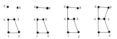
We can see from the images above that from filtration time 0 to 3, there are three parts formed by 4 edges and two vertices, thus dim0 is 1 and dim1 is 1. Then, at 3, there is an edge formed by the two vertices 5 and 6. Thus, from 3 until 5, dim0 is 2. Then, at filtration time 5, an edge connects the two parts, returning dim0 to 1. Finally, at filtration time 7, and edge connects the vertices of 6 and 3, leaving an abstract simplicial complex with dim0 as 1, and dim1 as 2, which is homeomorphic to the letter B. This is demonstrated by the image below.

The first image shows what is going on from 0 to 3.
The second image is from 3 to 5.
The third image is from 5 to 7.
The fourth image is from 7 on.

Figure 8

A simple form of a figure 8 represented by a Vietoris-Rips complex.

If we select the center to be at point (0,0), we can construct a simple figure 8. For this example, we will do so with only 7 vertices. The points are: (0,0),(1,1),(0,2),(-1,1),(-1,-1),(0,-2),(1,-1). We chose to insert the data as a point cloud and create a RipsStream that encases the data. In jPlex, the way to do this is as follows:

plex> double[][] figCoordinates = {{0,0},{1,1},{0,2},{-1,1},{-1,-1},{0,2},{1,-1}}; 

This inputs the coordinates of our figure, which will fit into the EuclideanArrayData constructor.

plex> pdatafig = Plex.EuclideanArrayData(figCoordinates); 
plex> ripsFig = Plex.RipsStream(0.001,3,1.8,pdatafig); 

(RipsStream is a type of stream that seems easily used here. The format for a RipsStream is given in the tutorial, however 1.8 is used as the maximum distance for an edge so that the dimension 1 is preserved)

plex> intervals = Plex.Persistence().computeIntervals(ripsFig); 
plex> Plex.plot(intervals, "ripsFig",5); 

The last line will print out results that look like this:

You can also check the Betti Numbers with the following command:

plex> Plex.FilterInfinite(intervals); Which will print out: 
<BN{1, 1}> 

This is not right. What has happened? Well, a simple error while inputting the vertices. Notice that we input vertex {0,2} twice instead of changing it to {0,-2} for the second vertex. When we correct this, we are left with the following barcodes:

Also, if we then check the Betti numbers, we get:

plex> Plex.FilterInfinite(intervals); Which will print out: 
<BN{1, 2}>

Another interesting thing to do is to look at the barcode when the maximum distance is increased to encase all data. We can do this by the same method as above by changing the maximum distance from 1.8 to say 4.

plex> double[][] figCoordinates = {{0,0},{1,1},{0,2},{-1,1},{-1,-1},{0,-2},{1,-1}}; 
plex> pdatafig = Plex.EuclideanArrayData(figCoordinates); 
plex> ripsFig = Plex.RipsStream(0.001,3,4,pdatafig); 
plex> intervals = Plex.Persistence().computeIntervals(ripsFig); 
plex> Plex.plot(intervals, "ripsFig",5); 

800px

As you can see, as the distance between points increases, the Dim 1 Homology appears and disappears, which demonstrates the importance of selecting the appropriate distance to consider a maximum.