This site is being phased out.
Integral: definition
We have realized:
- finding the position is equivalent to computing the area under the graph of the velocity,
- this computation will probably have to be carried out by approximating the area by vertical bars.
However, let's discuss what we mean by the area under the graph first.
In fact, what is the area?
Q: What is the area of a circle?
A: $\pi r^{2}$.
But how do we know?
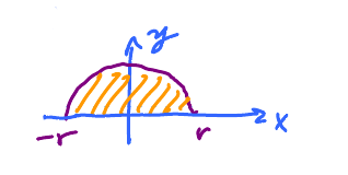
We interpret this as an area under the graph problem:
Find the area under the graph of $ y = f(x) = \sqrt{ r^{2} - x^{2} }$, multiply by 2. $$ \text{Upper half of the circle } = \text{ the graph of this function }$$ The actual computation will have to wait until Calc 2. For now, let's just say that if we do through the approximations and then take the limit, we'll arrive to $\pi r^{2}$.
This one is more manageable.
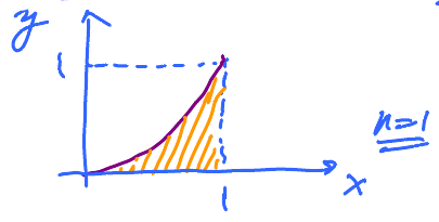
Example: Find the area under the graph of $y = f(x) = x^{2}$ from 0 to 1.
We will approximate by "sampling" our function at several values of $x$, $n$ of them.
Let's start with $n=1$ and pick the right end of the interval as the "sample" point.
$\bf{n=1}$
Compute $$f(1) = 1^{2} = 1,$$ so $$\text{Area } \approx 1 \cdot 1 = 1,$$ the whole square. We designate this as $R_1$: $$R_1=1.$$
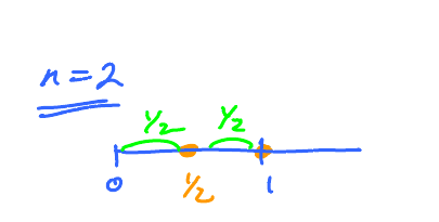
$\bf{n=2}$
| $x$ | $y = x^{2}$ | $\Delta x$ | Rectangle |
|---|---|---|---|
| $\frac{1}{2}$ | $\frac{1}{4}$ | $\frac{1}{2}$ | $\frac{1}{4}\cdot\frac{1}{2}$ |
| $1$ | $1$ | $\frac{1}{2}$ | $\frac{1}{2}\cdot 1$ |
| Add them |
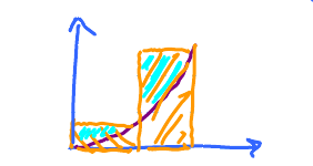
$$\text{Area } \approx \frac{1}{4}\cdot\frac{1}{2} + 1\cdot\frac{1}{2} = \frac{3}{4}\cdot\frac{1}{2} = \frac{5}{8}$$ ($\approx$ means "approximate", "estimate".)
We record this as: $$R_2=\frac{5}{8}.$$
Q: Do we underestimate or overestiamte the area?
A: Over.
Why?
There is extra area above the graph.
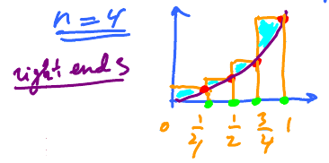
$\bf{n=4}$
$$\begin{gathered} \Delta x, \, a_{1} = \frac{1}{4}, \, a_{2} = \frac{1}{2}, \, a_{3} = \frac{3}{4}, \, a_{4} = 1 \\ \text{Area } \approx \frac{1}{4}\cdot\frac{1}{16} + \frac{1}{4}\cdot\frac{1}{4} + \frac{1}{4}\cdot\frac{9}{16} + \frac{1}{4}\cdot 1 \end{gathered} $$
We evaluate the function at the chosen points, "sample points". $$ \begin{aligned} &= \frac{1}{4}\left( \frac{1}{16} + \frac{4}{16} + \frac{9}{16} + \frac{16}{16}\right) \\ &= \frac{1}{4} \, \frac{30}{16} \approx 0.47 \end{aligned} $$ We record this as: $$R_4=.47.$$
Note: The exact answer is, in fact, $\frac{1}{3}$. That's the exact area under the graph of this parabola.
The "R" in $R_1,R_2,R_4$ stands for "right" as we chose the right ends of the intervals.
We continue with $n=8$, etc. We end up with a sequence of numbers. Then we take the limit. This limit is harder than what we have encountered as there are more and more items to add, $n$ items!
These sums are called Riemann sums. They
- approximate the exact area, and
- their limit is the exact area.
There are other ways to write Riemann sums if we choose other sample points.
Example: Again, find the area under $y = x^{2}$.
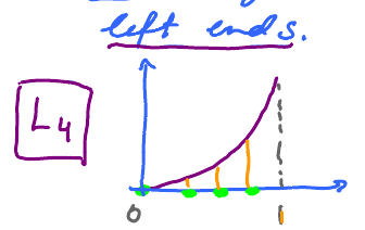
Pick new sample points: left ends this time.
Let $n=4$ (done above with right ends $R_{1}, \, R_{2}$, etc.).
$\Delta x = \frac{1}{4}$, 4 intervals. We choose: $$\underbrace{c_{1} = 0}_{\text{different}}, \, \underbrace{c_{2} = \frac{1}{4}, \, c_{3} = \frac{1}{2}, \, c_{4} = \frac{3}{4}}_{\text{same as before}} $$
$$\begin{aligned} \text{Area } &\approx \frac{1}{4} \cdot 0 + \frac{1}{4} \cdot \frac{1}{16} + \frac{1}{4}\cdot\frac{1}{4} + \frac{1}{4}\cdot\frac{9}{16} \\ &= \frac{1}{4} \left( 0 + \frac{1}{16} + \frac{1}{4} + \frac{9}{16} \right) \\ & = \frac{1}{4} \, \frac{19}{16} \approx 0.22. \end{aligned}$$
We record this as: $$L_4=.22,$$ recall $$R_4=.47.$$
This time we underestimate as there is extra area below the graph.
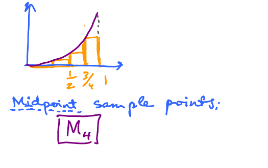
This time midpoint sample points:
Exercise: Compute $M_4$.
Next we consider the general setup for Riemann sums.
Given $y = f(x)$, continuous, defined on $[a,b], a < b$.
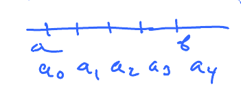
Given $n \geq 0$, $\text{integer } > 0$. Divide $[a,b]$ into $n$ intervals of equal length.
Then the intervals are: $$ [a_{0},a_{1}], [a_{1},a_{2}],\ldots , [a_{n-1},a_{n}].$$ Compute the length of each: $$\Delta x = \frac{b-a}{n}$$ Note: Recall and compare to: $$\frac{dy}{dx} = \lim_{\Delta x \to 0} \frac{\Delta y}{\Delta x}. $$
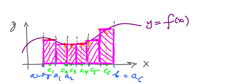
Given the sample points, one in each interval, $$ c_{1} \text{ in } [a_{0},a_{1}], \, c_{2} \text{ in } [a_{1},a_{2}],\ldots , c_{n} \text{ in } [a_{n-1},a_{n}].$$ Then the Riemann sum is $$f(c_{1})\Delta x + f(c_{2}) \Delta x + \ldots + f(c_{n})\Delta x. $$
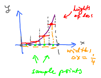
Observe that in each term of this sum: $$\underbrace{f(c_{k})}_{\text{Height of the 1st rectangle}} \cdot \overbrace{\Delta x}^{\text{width of rectangle}} $$ is the area of the corresponding rectangle
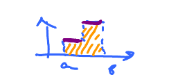
This is what the construction looks like with $n=6$ and arbitrary sample points:
Further, these are the rectangles:
$$\text{Riemann sum } = \text{ Total area of the rectangles}$$
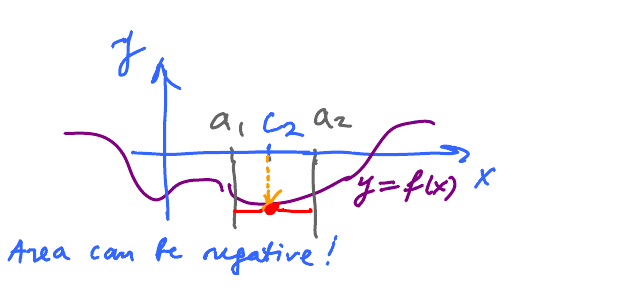
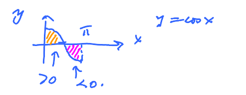
Observe that is this algebra $f(\underbrace{c_{i}}_{\text{sample point}})$ could be negative!
Then what's the meaning of $f(c_{2})\Delta x$?
It's the algebraic area of the rectangle.
To give an example, imagine again that $f$ is the speed. Then $f(c_{2})\Delta x$ is still distance "covered" but with the negative speed, you are moving in the opposite direction!
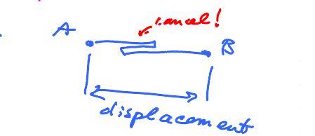
Conclusion: the Riemann sum, and the integral, captures not the distance covered but rather the displacement.
The difference is that you might be moving back at some point. In that case, the distances cancel each other.
Back to math, Riemann sum approximates the algebraic area "under" the graph or, more precisely, the area between the graph and the $x$-axis.
Example:
The area under the graph = 0. This follows from the symmetry of the graph.
The sigma notation
Consider again: $$RS = \underbrace{f(c_{1})\Delta x}_{\text{1 step}} + \underbrace{f(c_{2})\Delta x}_{\text{2 step}} + \ldots + \underbrace{f(c_{i})\Delta x}_{i\text{ step}} + \ldots + \underbrace{f(c_{n})\Delta x}_{n\text{ step}}. $$ This is cumbersome.
Let's look for a pattern.
Take the term in the middle $f(c_{i})\Delta x$. Then we observe that we can get any other term by plugging in $i = 1$, $i=2$, $\ldots$, $i=n$, respectively.
Then a better notation is $$\text{RS } = \sum_{i=1}^{n} f(c_{i})\Delta x.$$
We need this notation for integrals, but also consider:
$$1 + 2 + 3 + \ldots + 17 = \sum_{i=1}^{n} i.$$
More compact!
We can go back and "unwind" this notation: $$\sum_{i=1}^{17} i = \underbrace{1}_{i=1} + \underbrace{2}_{i=2} + \underbrace{3}_{i=3} + \ldots + \underbrace{17}_{i=17}$$
Example:
$$ \underbrace{0.5}_{i=1} + \underbrace{1}_{i=2} + \underbrace{1.5}_{i=3} + \ldots + \underbrace{17}_{i=34} = \sum_{i=1}^{17} \frac{i}{2}$$ Note: $i$ has to be an integer.
Example:
$$ 0 + 0.5 + 1.5 + \ldots + 17 = \sum_{i=0}^{17} \frac{i}{2}$$
Properties:
- $\sum\limits_{i=1}^{n} a = na = a + a + \ldots$ -- multiplication
- $ \sum\limits_{i=1}^{n} ca_{i} = c\sum\limits_{i=1}^{n} a_{i}$ -- factoring
- $ca_{1} + ca_{2} + \ldots + ca_{n} = c(a_{1} + a_{2} + \ldots + a_{n})$
-
- $\sum\limits_{i=1}^{n} \left( a_{i} + b_{i} \right) = \sum\limits_{i=1}^{n} a_{i} + \sum\limits_{i=1}^{n} b_{i} $
They correspond to the rules of integration ($\sum \to \int$).
Recall, $$ \text{RS} = \sum_{i=1}^{n} f(c_{i})\Delta x. $$
Finally, what if we "refine" the approximation and keep refining, i.e., $n \to \infty$?
The Riemann integral $\int_{a}^{b} f(x) dx$ is the limit of the Riemann sums as $n \to \infty$.
$$ \underbrace{\int_{a}^{b} f(x)\, dx}_{\text{the exact area under the graph}} = \lim_{n \to \infty}\underbrace{\sum_{i=1}^{n} f(c_{i})\Delta x}_{\text{RS, areas of bars}} $$
Observe that we have more and more terms here ($n \to \infty$). Meanwhile, $\Delta x \to 0$ as $\Delta x = \frac{b-a}{n} \to 0$ as $n \to \infty$.
If the limit exists, $f$ is called integrable.
Then "the area under the graph" makes sense!
Let's verify that the definition makes sense for the simplest function.
Example: Suppose $f(x) = 5$ for all $x$. Evaluate $\int_{0}^{2} f(x)\, dx$.
$$\begin{aligned} f(c_{i}) &= 5 \\ \Delta x &= \frac{2-0}{n} = \frac{2}{n}. \end{aligned}$$ Substitute.
The the Riemann sum is $$\begin{aligned} \sum_{i=1}^{n} f(c_{i}) \Delta x &= \sum_{i=1}^{n} \underbrace{5 \cdot \frac{2}{n}}_{\text{independent of } i} \\ &= 5 \, \frac{2}{n} \cdot n = 5 \cdot 2 = 10 \end{aligned}$$ The answer is correct!
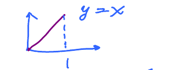
Example: This is a simpl function but it take a bit more to compute the are this way.
$$\begin{aligned} \int_{0}^{1} x \, dx &= \lim \, \text{RS} = \ldots \\ &= \frac{1}{2} \end{aligned} $$ (Exercise)
See Integral: properties.
