Functions of several variables

Overview of functions

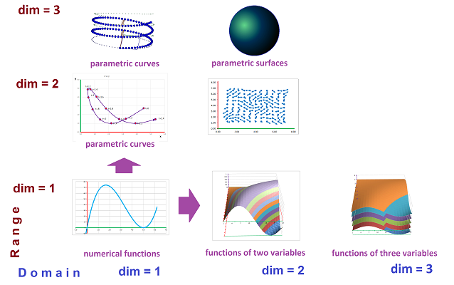
Let's review multidimensional functions. We have two axes: the dimension of the domain and the dimension of the range:

We covered the very first cell in Chapter 7. In Chapter 17, we made a step in the vertical direction and explored the first column of this table. It is now time to move to the right. We retreat to the first cell because the new material does not depend on the material of Chapter 17 -- or vice versa, even though they do interact via compositions. We will not jump diagonally!

We need to appreciate however the different challenges these two steps present. Every two numerical functions make a planar parametric curve and, conversely, every planar parametric curve is just a pair numerical functions. On the other hand, we can see that the surface that is the graph of a function of two variables produces -- through cutting by vertical planes -- infinitely many graphs of numerical functions.

Note that the first cell has curves but not all of them because some of them fail the vertical line test -- such as the circle -- and can't be represented by graphs of numerical functions. Hence the need for parametric curves. Similarly, the first cell of the second column has surfaces but not all of them because some of them fail the vertical line test -- such as the sphere -- and can't be represented by graphs of functions of two variables. Hence the need for parametric surfaces, shown higher in this column. They are presented in Chapter 19.

We represent a function diagrammatically as a black box that processes the input and produces the output of whatever nature: $$\newcommand{\ra}[1]{\!\!\!\!\!\xrightarrow{\quad#1\quad}\!\!\!\!\!} \newcommand{\da}[1]{\left\downarrow{\scriptstyle#1}\vphantom{\displaystyle\int_0^1}\right.} % \begin{array}{ccccccccccccccc} \text{input} & & \text{function} & & \text{output} \\ x & \mapsto & \begin{array}{|c|}\hline\quad f \quad \\ \hline\end{array} & \mapsto & y \end{array}$$ Let's compare the two: $$\newcommand{\ra}[1]{\!\!\!\!\!\xrightarrow{\quad#1\quad}\!\!\!\!\!} \newcommand{\da}[1]{\left\downarrow{\scriptstyle#1}\vphantom{\displaystyle\int_0^1}\right.} % \begin{array}{rcccl} \text{} & & \text{parametric } & & \text{} \\ \text{input} & & \text{curve} & & \text{output} \\ t & \mapsto & \begin{array}{|c|}\hline\quad F \quad \\ \hline\end{array} & \mapsto & X\\ {\bf R}& &&&{\bf R}^m\\ \text{number}& &&&\text{point or vector} \end{array}\quad \begin{array}{rcccl} \text{} & & \text{function of} & & \text{} \\ \text{input} & & \text{two variables} & & \text{output} \\ X & \mapsto & \begin{array}{|c|}\hline\quad f \quad \\ \hline\end{array} & \mapsto & z\\ {\bf R}^m& &&&{\bf R}\\ \text{point or vector}& &&&\text{number} \end{array}$$ They can be linked up and produce a composition...

But our interest is the latter starting with dimension $m=2$:

The main metaphor for a function of two variables will remain to be terrain:

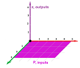
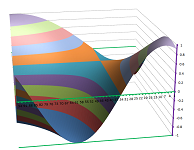
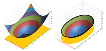
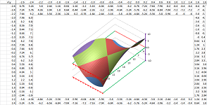
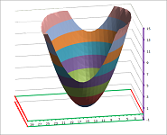
Here, every pair $X=(x,y)$ represents a location on a map and $z=f(x,y)$ is the elevation of the terrain at that location. This is how it is plotted by a spreadsheet:

Now calculus.

One subject of calculus is change and motion and, among others, we will address the question: if a drop of water land on this surface, in what direction will it flow? We will also consider the issue of the rate of change of the function -- in any direction.

Secondly, calculus studies tangency and linear approximations and, among others, we will address the question: if we zoom in on a particular location on the surface, what does it look like? The short answer is: like a plane. It is discussed in the next section.

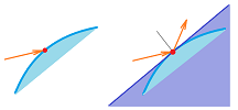
Examples of this issue have been seen previously. Indeed, recall that the Tangent Problem asks for a tangent line to a curve at a given point. It has been solved for parametric curves in Chapter 17. However, in real life we see surfaces rather than curves. The examples are familiar.

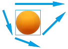
Example. In which direction a radar signal will bounce off a plane when the surface of the plane is curved?

In what direction will light bounce off a curved mirror?

What if it is a whole building?

$\square$

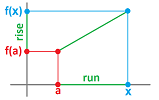
Recall the $1$-dimensional case. The difference quotient of a function $y=f(x)$ at $x=a$ is defined as the slope of the line that connects $(a,f(a))$ to the next point $(x,f(x))$: $$\frac{\Delta f}{\Delta x}=\frac{f(x)-f(a)}{x-a}.$$

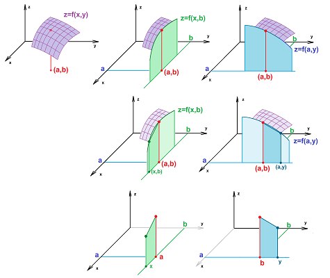
Now, let's see how this plan applies to functions of two variables $z=f(x,y)$. If we are interested in point $(a,b,f(a,b))$ on the graph of $f$, we still plot the line that connects this point to the next point on the grid. There are two point this time; they lie in the $x$- and the $y$-directions from $(a,b)$, i.e., $(x,b)$ and $(a,y)$ with $x\ne a$ and $y\ne b$.

The two slopes in these two directions are the two difference quotients, with respect to $x$ and with respect to $y$: $$\frac{\Delta f}{\Delta x}=\frac{f(x,b)-f(a,b)}{x-a} \text{ and } \frac{\Delta f}{\Delta y}=\frac{f(a,y)-f(a,b)}{y-b}.$$

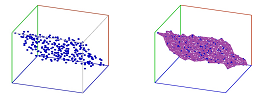
When done with every pair of nodes on the graph, the result is a mesh of triangles:

Furthermore, if the surface is the graph of a continuous function and we zoom in closer and closer on a particular point, we might expect the surface to start to look more and more straight like a plane.

Linear functions and planes in ${\bf R}^3$

We will approach the issue in a manner analogous to that for lines.

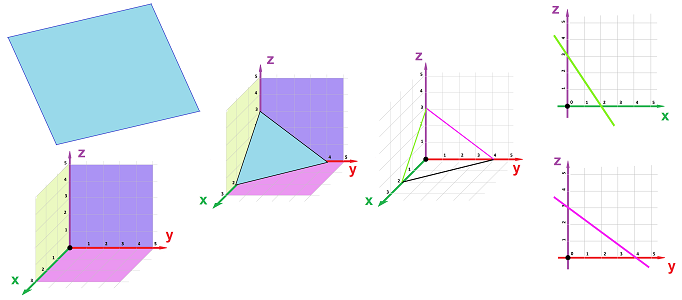
The standard, slope-intercept, form of the equation of a line in the $xy$-plane is: $$y=mx+p.$$ A similar, also in some sense slope-intercept, form of the equation of a plane in ${\bf R}^3$ is: $$z=mx+ny+p.$$ Indeed, if we substitute $x=y=0$ we have $z=p$.

Then $p$ is the $z$-intercept! In what sense are $m$ and $n$ slopes? Let's substitute $y=0$ first. We have $z=mx+p$, an equation of a line -- in the $xz$-plane. Its slope is $m$. Now we substitute $x=0$. We have $z=ny+p$, an equation of a line -- in the $yz$-plane. Its slope is $n$. Now, if we cut the plane with any plane parallel to the $xz$-plane, or respectively $yz$-plane, the resulting line has the same slope; for example: $$y=1\ \Longrightarrow\ z=mx+n+p;\quad x=1\ \Longrightarrow\ z=m+ny+p.$$

Therefore, we are justified to say that $m$ and $n$ are the slopes of the plane with respect to the variables $x$ and $y$ respectively: $$\begin{array}{llll} z=&m&\cdot x&+&n&\cdot y&+&p\\ &x\text{-slope}&&&y\text{-slope}&&&z\text{-intercept} \end{array}$$ Cutting with a horizontal plane also produces a line: $$z=1\ \Longrightarrow\ 1=mx+ny+p.$$

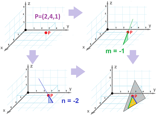
Next, the point-slope form of the equation of a line in the $xy$-plane is: $$y-b=m(x-a).$$ This is how we can plot this line. We start with the point $(a,b)$ in ${\bf R}^2$. Then we make a step along the $x$-axis with the slope $m$, i.e., we end up at $(a+1,b+m)$ or $(a+1/m,b+1)$, etc. These two points determine the line. There is a similar, also in some sense point-slope, form of the equation of a plane. This is the step we make: $$\begin{array}{r|l} \text{in }{\bf R}^2&\text{in }{\bf R}^3\\ \hline \begin{array}{rrr} \text{point }(a,b)\\ \text{slope }m \end{array}& \begin{array}{lll} \text{point }(a,b,c)\\ \text{slopes }m,n \end{array} \end{array}$$ This analogy produces the following formula: $$z-c=m(x-a)+n(y-b).$$ Expanding it takes us back to the point-slope formula.

This is how we can plot this plane. We start by plotting the point $(a,b,c)$ in ${\bf R}^3$. Now we treat one variable at a time. First, we fix $y$ and change $x$. From the point $(a,b,c)$, we make a step along the $x$-axis with the $x$-slope, i.e., we end up at $(a+1,b,c+m)$ or $(a+1/m,b,c+1)$, etc. The equation of this line is: $$z-c=m(x-a),\ y=b.$$ Second, we fix $x$ and change $y$. We make a step along the $y$-axis with the $y$-slope, i.e., we end up at $(a,b+1,c+n)$ or $(a,b+1/n,c+1)$, etc. The equation of this line is: $$x=a,\ z-c=n(y-b).$$ These three points (or those two lines through the same point) determine the plane. Below, we have $$(a,b,c)=(2,4,1),\ m=-1,\ n=-2.$$

What is a plane anyway? The planes we have considered so far are the graphs of (linear) functions of two variables: $$z=f(x,y)=mx+ny+p.$$ They have to satisfy the Vertical Line Test. Therefore, the vertical planes -- even the two $xz$- and $yz$-planes -- are excluded. This is very similar to the situation with lines and the impossibility to represent all lines in the standard form $y=mx+p$ and we need the general (implicit) equation of a line in ${\bf R}^2$: $$m(x-a)+n(y-b)=0.$$ The general (implicit) equation of a line in ${\bf R}^3$ is: $$m(x-a)+n(y-b)+k(z-c)=0.$$ Let's take a careful look at the left-hand side of this expression. There is a symmetry here over the three coordinates: $$\begin{array}{lll} m&\cdot&(x-a)+\\ n&\cdot&(y-b)+\\ k&\cdot&(z-c)=0 \end{array}\quad\leadsto\quad\left[ \begin{array}{lll}m\\n\\k\end{array}\right]\cdot \left[ \begin{array}{lll}x-a\\y-b\\z-c\end{array}\right]=0.$$ This is the dot product! The equation becomes: $$<m,n,k>\cdot <x-a,y-b,z-c>=0,$$ or even better: $$<m,n,k>\cdot \bigg( (x,y,z)-(a,b,c) \bigg) =0.$$ Finally a coordinate-free version: $$N\cdot (P-P_0)=0 \text{ or } N\cdot P_0P=0.$$ Here we have in ${\bf R}^3$:

• $P$ is the variable point,
• $P_0$ is the fixed point, and
• $N$ is any vector that somehow represents the slope of the plane.

The meaning of the vector $N$ is revealed once we remember that the dot product of two vectors is $0$ if and only if they are perpendicular.

These vectors are like bicycle's spokes to the hub $N$. This idea gives us our definition.

Definition. Suppose a point $P_0$ and a non-zero vector $N$ are given. Then the plane through $P_0$ with normal vector $N$ is the collection of all points $P$ -- and $P_0$ itself -- that satisfy: $$P_0P\perp N.$$

This definition gives us different results in different dimensions: $$\begin{array}{llll} \text{dimension}&\text{ambient space}&\text{“hyperplane”}&\\ \hline 2&{\bf R}^2&{\bf R}^1&\text{line}\\ 3&{\bf R}^3&{\bf R}^2&\text{plane}\\ 4&{\bf R}^4&{\bf R}^3&\text{--}\\ ...&...&...&...\\ \end{array}$$ A hyperplane is something very “thin” relative the whole space but not as thin as, say, a curve.

This wide applicability shows that learning the dot product really pays off!

We will need this formula to study parametric surfaces later. In this chapter we limit ourselves to functions of several variables and, therefore, non-vertical planes. What makes a plane non-vertical? A non-zero vertical component of the normal vector. Since length don't matter here (only the angles), we can simply assume that this component is equal to one: $$N=<m,n,1>.$$ Then the equation of a plane simplifies: $$0=N\cdot (P-P_0)=<m,n,1>\cdot<x-a,y-b,z-c>=m(x-a)+n(y-b)+z-c,$$ or the familiar $$z=c+m(x-a)+n(y-b).$$ In the vector notation, we have: $$z=c+M\cdot (Q-Q_0).$$ In case of dimension $2$ we have here:

• $Q=(x,y)$ is the variable point,
• $Q_0=(a,b)$ is the fixed point, and
• $M=<m,n>$ is the vector the components of which are the two slopes of the plane.

This is a linear function: $$z=f(x,y)=c+m(x-a)+n(y-b)=p+mx+ny,$$ and $M=<m,n>$ is called the gradient of $f$.

An example of a non-linear function

What makes a function linear? The implicit answer has been: the variable can only be multiplied by a constant and added to a constant. The first part of the answer still applies, even to functions of many variables as it prohibits multiplication by another variable. You can still add them.

The non-linearity of a function of two variables is seen as soon as it is plotted -- it's not a plane -- but it also suffices to limit its domain.

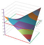
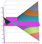
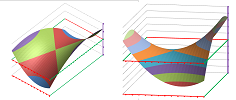
So, this function isn't linear: $$f(x,y)=xy.$$ In fact, $xy=x^1y^1$ is seen as quadratic if we add the powers of $x$ and $y$: $1+1=2$. We come to the same conclusion when we limit the domain of the function to the line $y=x$ in the $xy$-plane; using $y=x$ s a substitution we arrive to a function of one variable: $$g(x)=f(x,x)=x\cdot x=x^2.$$ So, the part of the graph of $f$ that lies exactly above the line $y=x$ is a parabola. And so is the part that lies above the line $y=-x$; it's just open down instead of up: $$h(x)=f(x,-x)=x\cdot (-x)=-x^2.$$ These two parabolas have a single point in common and therefore make up the essential part of a saddle point:

The former parabola gives room for the horse's front and back while the latter for the horseman's legs.

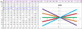
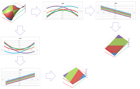
A simpler way to limit the domain is to fix one independent variable at a time. We fix $y$ first: $$\begin{array}{lrl} \text{plane}&\text{equation}&\text{curve}\\ \hline y=2&z=x\cdot 2&\text{line with slope }2\\ y=1&z=x\cdot 1&\text{line with slope }1\\ y=0&z=x\cdot 0=0&\text{line with slope }0\\ y=-1&z=x\cdot (-1)&\text{line with slope }1\\ y=-2&z=x\cdot (-2)&\text{line with slope }-2\\ \end{array}$$ The view shown below is from the direction of the $y$-axis:

The data for each line comes from the $x$-column of the spreadsheet and one of the $z$-columns. These lines give the lines of elevation of this terrain in a particular, say, east-west direction. This is equivalent to cutting the graph by a vertical plane parallel to the $xz$-plane.

We fix $x$ second: $$\begin{array}{lrl} \text{plane}&\text{equation}&\text{curve}\\ \hline x=2&z=2\cdot y&\text{line with slope }2\\ x=1&z=1\cdot y&\text{line with slope }1\\ x=0&z=0\cdot y=0&\text{line with slope }0\\ x=-1&z=(-1)\cdot y&\text{line with slope }1\\ x=-2&z=(-2)\cdot y&\text{line with slope }-2\\ \end{array}$$ This is equivalent to cutting the graph by a vertical plane parallel to the $yz$-plane. The view shown below is from the direction of the $x$-axis:

The data for each line comes from the $y$-row of the spreadsheet and one of the $z$-rows. These lines give the lines of elevation of this terrain in a particular, say, north-south direction.

Thus the surface of this graph is made of these straight lines! It's a potato chip:

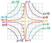
Another way to analyze the graph is to limit the range instead of the domain. We fix the dependent variable this time: $$\begin{array}{lrl} \text{elevation}&\text{equation}&\text{curve}\\ \hline z=2&2=x\cdot y&\text{hyperbola}\\ z=1&1=x\cdot y&\text{hyperbola}\\ z=0&0=x\cdot y&\text{the two axes}\\ z=-1&-1=x\cdot y&\text{hyperbola}\\ z=-2&-2=x\cdot y&\text{hyperbola} \end{array}$$ The result is a family of curves:

Each is labelled with the corresponding value of $z$, two branches for each. These lines are the lines of equal elevation of this terrain.

We can see who these lines come from cutting the graph by a horizontal plane (parallel to the $xy$-plane).

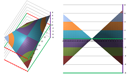
We can use them to reassemble the surface by lifting each to the elevation indicated by its label:

In the meantime, the colored parts of the graph correspond to intervals of outputs.

This surface presented here is called the hyperbolic paraboloid.

Graphs

Definition. The graph of a function of one variable $z=f(x)$ is the set of all points in ${\bf R}^{2}$ of the form $(x,f(x))$.

In spite of a few exceptions, the graphs of the function of one variable have been curves.

Definition. The graph of a function of two variables $z=f(x,y)$ is the set of all points in ${\bf R}^{3}$ of the form $(x,y,f(x,y))$.

In spite of possible exceptions, the graphs of functions of two variables we encounter will probably be surfaces.

It is important to remember that the theory of functions of several variables include that of the functions of one variable! The formula for $f$, for example, might have no mention of $y$ such as for example $z=f(x,y)=x^3$. The graph of such a function will be feature-less, i.e., constant, in the $y$-direction. It will look as if made of planks like a park bench:

In fact, the graph can be acquired from the graph of $z=x^2$ (the curve) by shifting it in the $y$-direction producing the surface:

In the last section we fixed one independent variable at a time making a function of two variables a function of one variable subject to the familiar methods. The idea applies to higher dimensions.

Definition. Suppose $z=f(x_1,...,x_n)$ is a function of several variables, i.e., $x_1,...,x_n$ and $z$ are real numbers. Then for each value of $k=1,2,...,n$ and any collection of numbers $x_i=a_i,\ i\ne k$, the numerical function defined by: $$z=h(x)=f(a_1,...,a_{k-1},x,a_{k+1},...,a_n),$$ is called a variable function of $f$. When $n=2$, its graph is called a variable curve.

We thus fix all variables but one making the function of $n$ variables a function of a single variable.

Exercise. What happens when $n=1$?

Meanwhile, fixing the value of the dependent variable doesn't have to produce a new function. The result is instead an implicit relation. The idea applies to higher dimensions too.

Definition. Suppose $z=f(X)$ is a function of several variables, i.e., $X$ belongs to some ${\bf R}^n$ and $z$ is a real number. Then for each value of $z=c$, the subset $$\{X:\ f(X)=c\}$$ of ${\bf R}^n$ is called a level set of $f$.

When $n=2$, it is informally called a level curve or a contour curve.

Exercise. What happens when $n=1$?

In general, a level set doesn't have to be a curve as the example of $f(x,y)=1$ shows.

Theorem. Level sets don't intersect.

Proof. It follows from the Vertical Line Test. $\blacksquare$

Exercise. Provide the proof.

Example. Let's consider: $$f(x,y)=\sqrt{x^2+y^2}.$$ The level curves are implicit curves and they are plotted point by point...

...unless we recognize them: $$c=\sqrt{x^2+y^2}\ \Longrightarrow\ c^2=x^2+y^2.$$ They are circles! This surface is a half of a cone. How do we know it's a cone and not another shape? We limit the domain to this line on the $xy$-plane: $$y=mx\ \Longrightarrow\ z=\sqrt{x^2+(mx)^2}=\sqrt{1+m}|x|.$$ These are V-shaped curves. $\square$

Example. Consider this function of two variables: $$f(x,y)=y^2-x^2.$$ Its level curves are hyperbolas again just as in the first example.

This is the familiar saddle point from the last section. Its variable curves are different simply because the angle of the graph relative to the axes is different. $\square$

Example. If we replace $-$ with $+$, the function of two variables becomes $$f(x,y)=y^2+x^2$$ with a very different graph; it has an extreme point. The variable curves are still parabolas but both point upward this time:

The level curves $$y^2+x^2=c$$ are circles except when $c=0$ (a point) or $c<0$ (empty). They don't grow uniformly, as with the cone, with $c$ however. The surface is called the paraboloid of revolution. One of the parabolas that passes through zero is rotated around the $z$-axis producing this surface. $\square$

The method of level curves has been used for centuries to create actual maps, i.e., $2$-dimensional visualizations of $3$-dimensional terrains.

The collection of all level curves is called the contour map of the function. We will see that zooming in on any point of the contour map is either a generic point with parallel level curves or a singular point exemplified by a saddle point and an extreme point.

The singular points are little islands in the sea of generic points...

Example. Suppose $z=f(x,y)$ is a function of two variables, then for each value of $z=c$, the subset $$\{(x,y):\ f(x,y)\le c\}$$ of the plane is called a sub-level set of $f$. These sets are used to convert gray-scale images to binary:

This operation is called “thresholding”. $\square$

Thus, the variable curves are the result of restricting the domain of the function while the level curves are the result of restricting the image. Either method is applied in hope of simplifying the function to the degree that will make is subject to the tool we already have. However, the original graph is made of infinitely many of those...

Informally, the meaning of the domain is the same: the set of all possible inputs.

Definition. The natural domain of a function $z=f(X)$ is the set of all $X$ in ${\bf R}^n$ for which $f(X)$ makes sense.

Just as before, the issue is that of division by zero, square roots, etc. The difference comes from the complexity of the space of inputs: the plane (and further ${\bf R}^n$) vs. the line.

Example. The domain of the function $$f(x,y)=\frac{1}{xy}$$ is the whole plane minus the axes.

$\square$

Example. The domain of the function $$f(x,y)=\sqrt{x-y}$$ is the half of the plane given by the inequality $y\le x$.

$\square$

Example. The domain of the function that represents the magnitude of the gravitational force is all points but $0$:

It is a multiple of the function: $$f(X)=\frac{1}{d(X,0)}.$$ $\square$

Exercise. Provide the level and the variable curves for the function that represents the magnitude of the gravitational force.

Definition. The graph of a function $z=f(X)$, where $X$ belongs to ${\bf R}^{n}$, is the set of all points in ${\bf R}^{n+1}$ so that the first $n$ coordinates are those of $X$ and the last is $f(X)$.

We have used the restriction of the image and the level curves that come from it as a tool of reduction. We reduce the study of a complex object -- the graph of $z=f(x,y)$ -- to a collection of simpler ones -- implicit curves $c=f(x,y)$. The idea is even more useful in the higher dimensions. In fact, we can't simply plot the graph of a function of three variables anymore -- it is located in ${\bf R}^4$ -- as we did for functions of two variables. The level sets -- level surfaces -- is the best way to visualize it. We can also restrict the domain instead by fixing one variable at a time and plot the graphs of the variable functions of two variables.

The domains of functions of three variables are in our physical space. They may represent:

• the temperature or the humidity,
• the air or water pressure,
• the magnitude of a force (such as gravitation), etc.

Example. The level sets of a linear function $$f(x,y,z)=A+mx+ny+kz.$$ are planes: $$d=A+mx+ny+kz.$$ These planes located in $xyz$-space are all parallel to each other because they have the same normal vector $<m,n,k>$. The variable functions aren't that different; let's fix $z=c$: $$d=f(x,y,c)=h(x,y)=A+mx+ny+kc.$$ For all values of $c$, these planes located in $xyu$-space are also parallel to each other because they have the same normal vector $<m,n,1>$. $\square$

Example. We start with a familiar function of two variables, $$f(x,y)=\sin(xy).$$ and just subtract $z$ as the third producing a new function of three variables: $$h(x,y,z)=\sin(xy)-z.$$ Then every of its level sets is given by: $$d=\sin(xy)-z,$$ for some real $d$. What is this? We can make the relation explicit: $$z=\sin(xy)-d,$$ Nothing but the graph of $f$ shifted down (and up) by $d$!

In this sense, they are parallel to each other. The function is growing as we move in the direction of $z$. Now, if we fix an independent variable of $h$, say $z=c$, we have a function of two variables: $$g(x,y)=\sin(xy)-c.$$ The graphs are the same. $\square$

Example. Let's consider this function of three variables: $$f(x,y,z)=\sqrt{x^2+y^2+z^2}.$$ Then every of its level sets is given by this implicit equation: $$d^2=x^2+y^2+z^2,$$ for some real $d$. Each is an equation of the sphere of radius $|d|$ centered at $0$ (and the origin itself when $d=0$). They are concentric!

The radii also grow uniformly with $d$ and, therefore, these surfaces are not are parallel to each other. So, the function is growing -- and at a constant rate -- as we move in any direction away from $0$. What is this function? It's the distance function itself: $$f(X)=f(x,y,z)=\sqrt{x^2+y^2+z^2}=||X||.$$

The graph of the magnitude of the gravitational force also has concentric spheres are level surfaces but the radii do not change uniformly with $d$. The value of the function is decreasing. $\square$

This is best we can do with functions of three variables. Beyond $3$ variables, we are out of dimensions...

The approach via fixing the independent variables is considered later.

Limits

We now study small scale behavior of functions; we zoom in on a single point of the graph. Just as in the lower dimensions, one of the most crucial properties of a function is the integrity of its graph: is there a break or a cut or a hole? For example, if we think of the graph as a terrain, is there a vertical drop?

We approach the issue via the limits.

In spite of all the differences between the functions we have seen -- such as parametric curves vs. functions of several variables -- the idea of limit is identical: as the input approaches a point, the output is also forced to approach a point. This is the context with the arrow “$\to$” to be read as “approaches”: $$\begin{array}{cccc} &\text{numerical functions}\\ &y=f(x)\to l\text{ as }x\to a\\ \text{parametric curves} && \text{functions of several variables}\\ Y=F(t)\to L\text{ as }t\to a && z=f(X)\to l\text{ as }X\to A\\ \end{array}$$ We use lower case for scalars and upper case for anything multi-dimensional (point or vectors). We then see how the complexity shifts from the output to the input. And so does the challenge of multi-dimensionality. We are ready though; this is the familiar meaning of convergence of a sequence in ${\bf R}^m$ to be used throughout: $$X_n\to A\ \Longleftrightarrow\ d(X_n,A)\to 0 \text{ or }||X_n-A||\to 0.$$

Definition. The limit of a function $z=f(A)$ at a point $X=A$ is defined to be the limit $$\lim_{n\to \infty} f(X_n)$$ considered for all sequences $\{X_n\}$ within the domain of $f$ excluding $A$ that converge to $A$, $$A\ne X_n\to A \text{ as } n\to \infty,$$ when all these limits exist and are equal to each other. In that case, we use the notation: $$\lim_{X\to A} f(X).$$ Otherwise, the limit does not exist.

We use this construction to understand what is happening to $z=f(X)$ when a point $X$ is in the vicinity of a chosen point $X=A$, where $f$ might be undefined. We start with an arbitrary sequence on the $xy$-plane that converges to this point, $X_n\to A$, then go vertically from each of these point to find the corresponding points on the graph of the function, $(X_n,f(X_n))$, and finally plot the output values (just numbers) on the $z$-axis, $z_n=f(X_n)$.

Is there a limit of this sequence? What about other sequences? Are all these limits the same?

The ability to approach the point from different directions had to be dealt with even for numerical functions: $$\operatorname{sign}(x)\to -1 \text{ as } x\to 0^- \text{ but } \operatorname{sign}(x)\to 1 \text{ as } x\to 0^+.$$ In the multi-dimensional case things are even more complicated as we can approach a point on the plane from infinitely many directions.

Example. It is easy to come up with an example of a function that has different limits from different directions. We take one that will be important in the future: $$\lim_{(x,y)\to (0,0)}\frac{|2x+y|}{\sqrt{x^2+y^2}}.$$ By the way, this is how one might try to calculate the “slope” (rise over the run) at $0$ of the plane $z=2x+y$. First, we approach along the $x$-axis, i.e., $y$ is fixed at $0$: $$\lim_{x\to 0}\frac{|2x+0|}{\sqrt{x^2+0^2}}=\lim_{x\to 0}\frac{|2x|}{|x|}=2.$$ Second, we approach along the $y$-axis, i.e., $x$ is fixed at $0$: $$\lim_{y\to 0}\frac{|2\cdot 0+y|}{\sqrt{0^2+y^2}}=\lim_{y\to 0}\frac{|y|}{|y|}=1.$$ There can't be just one slope for a plane... $\square$

Things might be bad in an even more subtle way.

Example. Not all functions of two variables have graphs like the one above... Let's consider this function: $$f(x,y)=\frac{x^2y}{x^4+y^2}.$$ and its limit $(x,y)\to (0,0)$. Does it exist? It all depends on how $X$ approaches $A=0$:

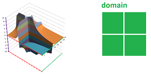
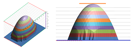
The two green horizontal lines indicate that we get $0$ if we approach $0$ from either the $x$ or the $y$ direction. That's the horizontal cross we see on the surface (just like the one in the hyperbolic paraboloid). In fact, any (linear) direction is OK: $$y=mx\ \Longrightarrow\ f(x,mx)=\frac{x^2mx}{x^4+(mx)^2}=\frac{mx^3}{x^4+m^2x^2}=\frac{m}{x+m^2/x}\to 0 \text{ as }x\to 0.$$ So, the limits from all directions are the same! However, there seems to be two curved cliffs on left and right visible form above... What is we approach $0$ along, instead of a straight line, a parabola $y=x^2$? The result is surprising: $$y=x^2\ \Longrightarrow\ f(x,x^2)=\frac{x^2x^2}{x^4+(x^2)^2}=\frac{x^4}{2x^4}=\frac{1}{2}.$$ This is the height of the cliffs! So, this limit is different from the other and, according to our definition, the limit of the function does not exist: $$\lim_{(x,y)\to (0,0)}\frac{x^2y}{x^4+y^2}\ DNE.$$ In fact, the illustration created by the spreadsheet attempts to make an unbroken surface from these points while in reality there is no passage between the two cliffs as we just demonstrated.

$\square$

So, not only we have to approach the point from all directions at once but also along any possible path.

A simpler but very important conclusion is that studying functions of several variables one variable at a time might be insufficient or even misleading.

A special note about the limit of a function at a point that lies on the boundary of the domain... It doesn't matter! The case of one-sided limits at $a$ or $b$ of the domain $[a,b]$ is now included in our new definition.

The algebraic theory of limits is almost identical to that for numerical functions. There are as many rules because whatever you can do with the outputs you can do with the functions.

We will use the algebraic properties of the limits of sequences -- of numbers -- to prove virtually identical facts about limits of functions.

Theorem (Algebra of Limits of Sequences). Suppose $a_n\to a$ and $b_n\to b$. Then $$\begin{array}{|ll|ll|} \hline \text{SR: }& a_n + b_n\to a + b& \text{CMR: }& c\cdot a_n\to ca& \text{ for any real }c\\ \text{PR: }& a_n \cdot b_n\to ab& \text{QR: }& a_n/b_n\to a/b &\text{ provided }b\ne 0\\ \hline \end{array}$$

Each property is matched by its analog for functions.

Theorem (Algebra of Limits of Functions). Suppose $f(X)\to a$ and $g(X)\to b$ as $X\to A$ . Then $$\begin{array}{|ll|ll|} \hline \text{SR: }& f(X)+g(X)\to a+b & \text{CMR: }& c\cdot f(X)\to ca& \text{ for any real }c\\ \text{PR: }& f(X)\cdot g(X)\to ab& \text{QR: }& f(X)/g(X)\to a/b &\text{ provided }b\ne 0\\ \hline \end{array}$$

Note that there were no PR or QR for the parametric curves...

Let's consider them one by one.

Now, limits behave well with respect to the usual arithmetic operations.

Theorem (Sum Rule). If the limits at $A$ of functions $f(X),g(X)$ exist then so does that of their sum, $f(P) + g(P)$, and the limit of the sum is equal to the sum of the limits: $$\lim_{X\to A} \big( f(X) + g(X) \big) = \lim_{X\to A} f(X) + \lim_{X\to A} g(X).$$

Since the outputs and the limits are just numbers, in the case of infinite limits we follow the same rules of the algebra of infinities as in Chapter 5: $$\begin{array}{lll} \text{number } &+& (+\infty)&=+\infty\\ \text{number } &+& (-\infty)&=-\infty\\ +\infty &+& (+\infty)&=+\infty\\ -\infty &+& (-\infty)&=-\infty\\ \end{array}$$

The proofs of the rest of the properties are identical.

Theorem (Constant Multiple Rule). If the limit at $X=A$ of function $f(X)$ exists then so does that of its multiple, $c f(X)$, and the limit of the multiple is equal to the multiple of the limit: $$\lim_{X\to A} c f(X) = c \cdot \lim_{X\to A} f(X).$$

Theorem (Product Rule). If the limits at $a$ of functions $f(X) ,g(X)$ exist then so does that of their product, $f(X) \cdot g(X)$, and the limit of the product is equal to the product of the limits: $$\lim_{X\to A} \big( f(X) \cdot g(X) \big) = \left(\lim_{X\to A} f(X)\right)\cdot\left( \lim_{X\to A} g(X)\right).$$

Theorem (Quotient Rule). If the limits at $X=A$ of functions $f(X) ,g(X)$ exist then so does that of their ratio, $f(X) / g(X)$, provided $\lim_{X\to A} g(X) \ne 0$, and the limit of the ratio is equal to the ratio of the limits: $$\lim_{X\to A} \left(\frac{f(X)}{g(X)}\right) = \frac{\lim\limits_{X\to A} f(X)}{\lim\limits_{X\to A} g(X)}.$$

Just as with sequences, we can represent these rules as commutative diagrams: $$\newcommand{\ra}[1]{\!\!\!\!\!\xrightarrow{\quad#1\quad}\!\!\!\!\!} \newcommand{\la}[1]{\!\!\!\!\!\xleftarrow{\quad#1\quad}\!\!\!\!\!} \newcommand{\da}[1]{\left\downarrow{\scriptstyle#1}\vphantom{\displaystyle\int_0^1}\right.} \newcommand{\ua}[1]{\left\uparrow{\scriptstyle#1}\vphantom{\displaystyle\int_0^1}\right.} \begin{array}{ccc} f,g&\ra{\lim}&l,m\\ \ \da{+}&SR &\ \da{+}\\ f+g & \ra{\lim}&\lim(f+g)=l+m \end{array}$$

Example. $$\lim_{(x,y)\to (0,0)}\frac{x^2+y^2}{x+y}=...$$ $\square$

We can take advantage of the fact that the domain ${\bf R}^m$ of $f$ can also be seen as made of vectors and vectors are subject to algebraic operations.

Theorem (Alternative formula for limits). The limit of a function $z=f(X)$ at $X=A$ is equal to $l$ if and only if $$\lim_{||H|| \to 0} f(A + H) = l.$$

The next result stands virtually unchanged from Chapter 6.

Theorem (Squeeze Theorem). If a function is squeezed between two functions with the same limit at a point, its limit also exists and is equal to the that number; i.e., if $$f(X) \leq h(X) \leq g(X) ,$$ for all $X$ within some distance from $X=A$, and $$\lim_{X\to A} f(X) = \lim_{X\to A} g(X) = l,$$ then the following limit exists and equal to that number: $$\lim_{X\to A} h(X) = l.$$

The easiest way to handle limits is coordinate-wise, when possible.

Theorem. If the limit of a function of several variables exists then it exists with respect to each of the variables; i.e., for any function $z=f(X)=f(x_1,...,x_m)$ and any $A=(a_1,...,a_m)$ in ${\bf R}^m$, we have $$\begin{array}{rll} f(X)\to l \text{ as }X\to A\\ \Longrightarrow& f(a_1,...,a_{k-1},x,a_{k+1},...,a_m)\to l \text{ as }x\to a_k \text{ for each } k=1,2,...,m. \end{array}$$

The converse isn't true!

Example. Recall that this function has limits at $(0,0)$ with respect to either of the variables: $$f(x,y)=\frac{x^2y}{x^4+y^2},$$ but the limit as $(x,y)\to (0,0)$ does not exist. $\square$

So, we have to establish that the limit exists -- in the “omni-directional” sense -- first and only then we can use limits with respect to every variable -- in the “uni-directional” sense -- to find this limit.

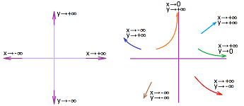
Now, the asymptotic behavior...

Definition. Given a function $z=f(X)$ and a point $A$ in ${\bf R}^n$, we say that $f$ approaches infinity at $A$ if $$\lim_{n\to \infty}f(x)=\pm\infty,$$ for any sequence $X_n\to A$ as $n\to \infty$. Then we use the notation: $$\lim_{X\to A}f(x)=\pm\infty .$$ The line $X=A$ located in ${\bf R}^{n+1}$ is then called a vertical asymptote of $f$.

Example (Newton's Law of Gravity). If $z=f(x,y,z)$ represents the magnitude of the force of gravity of an object located at the point $X=(x,y,z)$ relative to another object located at the origin, then we have: $$ \lim_{X \to 0} f (X)= \infty.$$ $\square$

Next, we can approach infinity in a number of ways too:

That's why we have to look at the distance to the origin.

Definition. For a function of several variables $z=f(X)$, we say that $f$ goes to infinity if $$f(X_n)\to \pm\infty,$$ for any sequence $X_n$ with $||X_n||\to \infty$ as $n\to \infty$. Then we use the notation: $$f(X) \to \pm\infty \text{ as }X\to \infty,$$ or $$\lim_{x\to\infty}f(x)=\pm\infty.$$

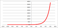
Example. We previously demonstrated the following: $$\lim_{x \to -\infty} e^{x} = 0, \quad \lim_{x \to +\infty} e^{x} = +\infty.$$

$\square$

We won't speak of horizontal asymptotes but the next idea is related.

Definition. Given a function $z=f(X)$, we say that $f$ approaches $z=d$ at infinity if $$\lim_{n\to \infty}f(X_n)=d,$$ for any sequence $X_n$ with $||X_n||\to \infty$ as $n\to \infty$. Then we use the notation: $$\lim_{X\to \infty}f(X)=d .$$

Example (Newton's Law of Gravity). If $z=f(x,y,z)$ represents the magnitude of the force of gravity of an object located at the point $X=(x,y,z)$ relative to another object located at the origin, then we have: $$ \lim_{X \to \infty} f (X)= 0.$$ $\square$

Continuity

The idea of continuity is identical to that for numerical functions or parametric cures: as the input approaches a point, the output is forced to approach the values of the function at that point. The concept flows from the idea of limit just as before.

Definition. A function $z=f(X)$ is called continuous at point $X=A$ if

• $f(X)$ is defined at $X=A$,
• the limit of $f$ exists at $A$, and
• the two are equal to each other:

$$\lim_{X\to A}f(X)=f(A).$$ Furthermore, a function is continuous if it is continuous at every point of its domain.

Thus, the limits of continuous functions can be found by substitution: $$\newcommand{\ra}[1]{\!\!\!\!\!\xrightarrow{\quad#1\quad}\!\!\!\!\!} \newcommand{\da}[1]{\left\downarrow{\scriptstyle#1}\vphantom{\displaystyle\int_0^1}\right.} % \begin{array}{|c|}\hline\quad \lim_{X\to A}f(X)=f(A) \quad \\ \hline\end{array} \text{ or } \begin{array}{|c|}\hline\quad f(X)\to f(A) \text{ as } X\to A.\quad \\ \hline\end{array} $$

Equivalently, a function $f$ is continuous at $a$ if $$\lim_{n\to \infty}f(A_n)=f(A),$$ for any sequence $X_n\to A$.

A typical function we encounter is continuous at every point of its domain.

Theorem. Suppose $f$ and $g$ are continuous at $X=A$. Then so are the following functions:

• 1. (SR) $f\pm g$,
• 2. (CMR) $c\cdot f$ for any real $c$,
• 3. (PR) $f \cdot g$, and
• 4. (QR) $f/g$ provided $g(A)\ne 0$.

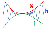
As an illustration, we can say that if the floor and the ceiling represented by $f$ and $g$ respectively of a cave are changing continuously then so is its height, which is $g-f$:

Or, if the floor and the ceiling ($f$ and $-g$) are changing continuously then so is its height ($g+f$). And so on.

There are two ways to compose a function of several variables with another function...

Theorem (Composition Rule I). If the limit at $X=A$ of function $z=f(X)$ exists and is equal to $l$ then so does that of its composition with any numerical function $u=g(z)$ continuous at $z=l$ and $$\lim_{X\to A} (g\circ f)(X) = g(l).$$

Proof. Suppose we have a sequence, $$X_n\to A.$$ Then, we also have another sequence, $$b_n=f(X_n).$$ The condition $f(X)\to l$ as $X\to A$ is restated as follows: $$b_n\to l \text{ as } n\to \infty.$$ Therefore, continuity of $g$ implies, $$g(b_n)\to g(l)\text{ as } n\to \infty.$$ In other words, $$(g\circ f)(X_n)=g(f(X_n))\to g(l)\text{ as } n\to \infty.$$ Since sequence $X_n\to A$ was chosen arbitrarily, this condition is restated as, $$(g\circ f)(X)\to g(l)\text{ as } X\to A.$$ $\blacksquare$

We can re-write the result as follows: $$\newcommand{\ra}[1]{\!\!\!\!\!\xrightarrow{\quad#1\quad}\!\!\!\!\!} \newcommand{\da}[1]{\left\downarrow{\scriptstyle#1}\vphantom{\displaystyle\int_0^1}\right.} % \begin{array}{|c|}\hline\quad \lim_{X\to A} (g\circ f)(X) = g(l)\Bigg|_{l=\lim_{X\to A} f(X)} \quad \\ \hline\end{array} $$ Furthermore, we have $$\newcommand{\ra}[1]{\!\!\!\!\!\xrightarrow{\quad#1\quad}\!\!\!\!\!} \newcommand{\da}[1]{\left\downarrow{\scriptstyle#1}\vphantom{\displaystyle\int_0^1}\right.} % \begin{array}{|c|}\hline\quad \lim_{X\to A} g\big( f(X) \big) = g\left( \lim_{X\to A} f(X) \right) \quad \\ \hline\end{array} $$

Theorem (Composition Rule II). If the limit at $t=a$ of a parametric curve $X=F(t)$ exists and is equal to $L$ then so does that of its composition with any function $z=g(X)$ of several variables continuous at $X=L$ and $$\lim_{t\to a} (g\circ F)(t) = g(L).$$

Proof. Suppose we have a sequence, $$t_n\to a.$$ Then, we also have another sequence, $$B_n=F(t_n).$$ The condition $F(t)\to L$ as $t\to a$ is restated as follows: $$B_n\to L \text{ as } n\to \infty.$$ Therefore, continuity of $F$ implies, $$g(B_n)\to g(L)\text{ as } n\to \infty.$$ In other words, $$(g\circ F)(t_n)=g(F(t_n))\to g(L)\text{ as } n\to \infty.$$ Since sequence $X_n\to A$ was chosen arbitrarily, this condition is restated as, $$(g\circ F)(t)\to g(L)\text{ as } t\to a.$$ $\blacksquare$

We can re-write the result as follows: $$\newcommand{\ra}[1]{\!\!\!\!\!\xrightarrow{\quad#1\quad}\!\!\!\!\!} \newcommand{\da}[1]{\left\downarrow{\scriptstyle#1}\vphantom{\displaystyle\int_0^1}\right.} % \begin{array}{|c|}\hline\quad \lim_{t\to a} (g\circ F)(t) = g(L)\Bigg|_{L=\lim_{t\to a} F(t)} \quad \\ \hline\end{array} $$ Furthermore, we have: $$\newcommand{\ra}[1]{\!\!\!\!\!\xrightarrow{\quad#1\quad}\!\!\!\!\!} \newcommand{\da}[1]{\left\downarrow{\scriptstyle#1}\vphantom{\displaystyle\int_0^1}\right.} % \begin{array}{|c|}\hline\quad \lim_{t\to a} g\big( F(t) \big) = g\left( \lim_{t\to a} F(t) \right) \quad \\ \hline\end{array} $$

Corollary. The composition $g\circ f$ of a function $f$ continuous at $x=a$ and a function $g$ continuous at $y=f(a)$ is continuous at $x=a$.

The easiest way to handle continuity is coordinate-wise, when possible.

Theorem. If a function of several variables is continuous then it is also continuous with respect to each of the variables.

The converse isn't true!

Example. Recall that this function is continuous at $(0,0)$ with respect to either of the variables: $$f(x,y)=\frac{x^2y}{x^4+y^2},$$ but the limit as $(x,y)\to (0,0)$ simply does not exist. $\square$

So, we have to establish continuity -- in the sense of the “omni-directional” limit -- first and only then we can use this fact to find facts about the continuity with respect to every variable -- in the “uni-directional” sense.

A special note about the continuity of a function at a point that lies on the boundary of the domain... Once again, it doesn't matter! The case of one-sided continuity at $a$ or $b$ of the domain $[a,b]$ is now included in our new definition.

The definition of continuity is purely local: only the behavior of the function in the, no matter how small, vicinity of the point matters. If the function is continuous on a whole set, what can we say about its global behavior?

Our understanding of continuity of numerical functions has been as the property of having no gaps in their graphs.

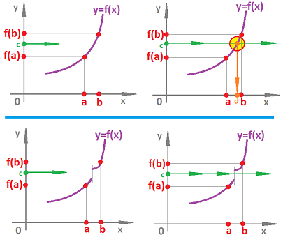
This idea is more precisely expressed by the following by the Intermediate Value Theorem:

• if a function $f$ is defined and is continuous on an interval $[a,b]$, then for any $c$ between $f(a)$ and $f(b)$, there is $d$ in $[a,b]$ such that $f(d) = c$.

An often more convenient way to state is:

• if the domain of a continuous function is an interval then so is its image.

Now the plane is more complex than a line and we can't limit ourselves to intervals. But what is the analog of an interval in a multidimensional space?

Theorem (Intermediate Value Theorem for functions of several variables). Suppose a function $f$ is defined and is continuous on a set that contains the path $C$ of a continuous parametric curve. Then the image of this path is an interval.

Proof. It follows from the Composition Rule II and the Intermediate Value Theorem for numerical functions. $\blacksquare$

The theorem says that there are no missing values in the image of such a set.

Exercise. Show that that the converse of the theorem isn't true.

A convenient re-statement of the theorem is below.

Corollary. The image of a path-connected set under a continuous function is an interval.

Recall that a function $f$ is called bounded on a set $S$ in ${\bf R}^n$ if its image is bounded, i.e., there is such a real number $m$ that $$|f(X)| \le m$$ for all $X$ in $S$.

Theorem. If the limit at $X=A$ of function $z=f(X)$ exists then $f$ is bounded on some open disk that contains $A$: $$\lim_{X\to A}f(X) \text{ exists }\ \Longrightarrow\ |f(X)| \le m$$ for all $X$ with $d(X,A)<\delta$ for some $\delta >0$ and some $m$.

Exercise. Prove the theorem.

The global version of the above theorem guarantees that the function is bounded under certain circumstances.

The version of the theorem for numerical functions is simply: a continuous on $[a,b]$ function is bounded.

But what is the multi-dimensional analog of a closed bounded interval?

We already know that a set $S$ in ${\bf R}^n$ is bounded if it fits in a sphere (or a box) of a large enough size: $$||x|| < Q \text{ for all } x \text{ in } S;$$ and a set in ${\bf R}^n$ is called closed if it contains the limits of all of its convergent sequences.

Theorem (Boundedness). A continuous on a closed bounded set function is bounded.

Proof. Suppose, to the contrary, that $x=f(X)$ is unbounded on set $S$. Then there is a sequence $\{X_n\}$ in $S$ such that $f(X_n)\to \infty$. Then, by the Bolzano-Weierstrass Theorem, sequence $\{X_n\}$ has a convergent subsequence $\{Y_k\}$: $$Y_k \to Y.$$ This point belong to $S$! From the continuity, it follows that $$f(Y_k) \to f(Y).$$ This contradicts the fact that $\{Y_k\}$ is a subsequence of a sequence that diverges to $\infty$. $\blacksquare$

Exercise. Why are we justified to conclude in the proof that the limit $Y$ of $\{Y_k\}$ is in $S$?

Is the image of a closed set closed? If it is, the function reaches its extreme values, i.e., the least upper bound $\sup$ and the greatest lower bound $\inf$.

Definition. Given a function $z=f(X)$. Then $X=D$ is called a global maximum point of $f$ on set $S$ if $$f(D)\ge f(X) \text{ for all } X \text{ in }S;$$ and $X=C$ is called a global minimum point of $f$ on set $S$ if $$f(C)\le f(X) \text{ for all } X \text{ in }S.$$ (They are also called absolute maximum and minimum points.) Collectively they are all called global extreme points.

Just because something is described doesn't mean that it can be found.

Theorem (Extreme Value Theorem). A continuous function on a closed bounded set in ${\bf R}^n$ attains its global maximum and global minimum values; i.e., if $z=f(X)$ is continuous on a bounded closed set $S$, then there are $C,D$ in $S$ such that $$f(C)\le f(X) \le f(D),$$ for all $X$ in $S$.

Proof. It follows from the Bolzano-Weierstrass Theorem. $\blacksquare$

Definition. Given a function $z=f(X)$. Then $X=M$ is called the global maximum value of $f$ on set $S$ if $$M\ge f(X) \text{ for all } X \text{ in }S;$$ and $y=m$ is called the global minimum value of $f$ on set $S$ if $$m\le f(X) \text{ for all } X \text{ in }S.$$ (They are also called absolute maximum and minimum values.) Collectively they are all called global extreme values.

Then the global max (or min) value is reached by the function at any of its global max (or min) points.

Note that the reason we need the Extreme Value Theorem is to ensure that the optimization problem we are facing has a solution.

We can define limits and continuity of functions of several variables without invoking limits of sequences. Let's re-write what we want to say about the meaning of the limits in progressively more and more precise terms. $$\begin{array}{l|ll} X&z=f(X)\\ \hline \text{As } X\to A, & \text{we have } y\to l.\\ \text{As } X\text{ approaches } A, & y\text{ approaches } l. \\ \text{As } \text{the distance from }X \text{ to } A \text{ approaches } 0, & \text{the distance from }y \text{ to } l \text{ approaches } 0. \\ \text{As } d(X,A)\to 0, & \text{we have } |y-l|\to 0.\\ \text{By making } d(X,A) \text{ as smaller and smaller},& \text{we make } |y-l| \text{ as small as needed}.\\ \text{By making } d(X,A) \text{ less than some } \delta>0 ,& \text{we make } |y-l| \text{ smaller than any given } \varepsilon>0. \end{array}$$

Definition. The limit of function $z=f(X)$ at $X=A$ is a number $l$, if exists, such that for any $\varepsilon >0$ there is such a $\delta> 0$ that $$0<d(X,A)<\delta \ \Longrightarrow\ |f(X)-l|<\varepsilon.$$

This is the geometric meaning of the definition: if $X$ is within $\delta$ from $A$, then $f(X)$ is supposed to be within $\varepsilon$ from $l$. In other words, this part of the graph fits between the two planes $\varepsilon$ away from the plane $z=l$.

The partial differences and difference quotients

We start with numerical differentiation of functions of several variables.

Example. We consider the function: $$f(x,y)=-x^2+y^2+xy.$$ For each $x$ in the left-most column and each $y$ in the top row, the corresponding value of the function is computed and placed in this table, just as before: $$\texttt{=R2C3*(R4C^2-RC2^2+R4C*RC2)}.$$

When plotted is recognized as a familiar hyperbolic paraboloid.

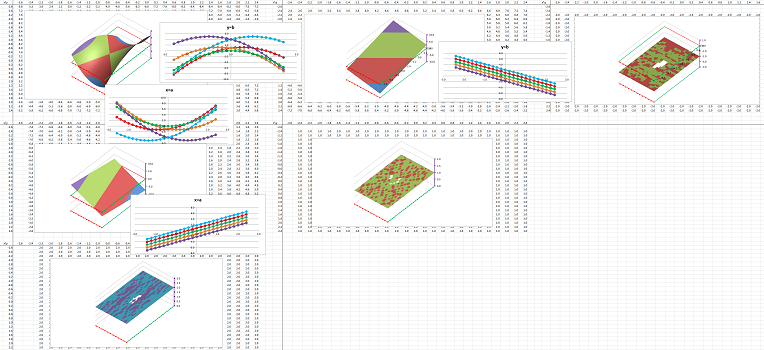
Below we outline the process of partial differentiation. The variable functions -- with respect to $x$ and $y$ -- are shown. These are the functions we will differentiate.

First, for each value of $y$ given in the top row, we compute the difference quotient function with respect to $x$ by going down the corresponding column and then placing these values on right in a new table (it is one row short in comparison to the original): $$\texttt{=(RC[-29]-R[-1]C[-29])/R2C1}.$$

Second, for each value of $x$ given in the left-most column, we compute the difference quotient function with respect to $y$ by going right the corresponding row and then placing these values below in a new table (it is one column short in comparison to the original). $$\texttt{=(R[-29]C-R[-29]C[-1])/R2C1}.$$

This is the summary:

The results are all straight lines equally spaced and in both cases they form planes. These planes are the graphs of the two new functions of two variables, the partial derivatives, the tables of which have been constructed. Some things don't change: just as in the one-dimensional case, the derivatives of quadratic functions are linear. $\square$

We deal with the change of the values of a function, $\Delta f$, relative to the change of its input variable. This time, there are two: $\Delta x$ and $\Delta y$.

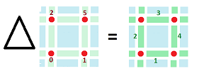
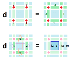
If we know only four values of a function of two variables (left), we can compute the differences $\Delta_x f$ and $\Delta_y f$ of $f$ along both horizontal and vertical edges (right): $$\begin{array}{rcccccccc} y+\Delta y:&f(x,y+\Delta y)&---&f(x+\Delta x,y+\Delta y)&&-\bullet-&\Delta_x f(s,y+\Delta y)&-\bullet-\\ &|&&|&&|&&|\\ t:&|&&|&\leadsto&\Delta_y f(x,t)&&\Delta_y f(x+\Delta x,t)\\ &|&&|&&|&&|\\ y:&f(x,y)&---&f(x+\Delta x,y)&&-\bullet-&\Delta_x f(s,y)&-\bullet-\\ &x&s&x+\Delta x&&x&s&x+\Delta x\\ \end{array}$$ As you can see, we subtract the values at the corners -- vertically and horizontally -- and place them at the corresponding edges. We then acquire the difference quotients by dividing by the increment of the corresponding variable: $$\leadsto\quad\begin{array}{cccccccc} -\bullet-&\frac{\Delta f}{\Delta x}(s,y+\Delta y)&-\bullet-\\ |&&|\\ \frac{\Delta f}{\Delta y}(x,t)&&\frac{\Delta f}{\Delta y}(x+\Delta x,t)\\ |&&|\\ -\bullet-&\frac{\Delta f}{\Delta x}(s,y)&-\bullet-\\ &x&s&x+\Delta x\\ \end{array}$$ Here and below we omit the subscripts in the fractions $\frac{\Delta_x f}{\Delta x}$ and $\frac{\Delta_y f}{\Delta y}$.

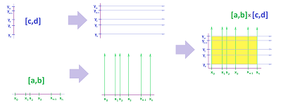
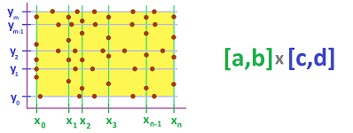
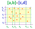
More generally, we build a partition $P$ of a rectangle $R=[a,b]\times [c,d]$ in the $xy$-plane. It is a combination of partitions of the intervals $[a,b]$ and $[c,d]$:

We start with a partition of an interval $[a,b]$ in the $x$-axis into $n$ intervals: $$ [x_{0},x_{1}],\ [x_{1},x_{2}],\ ... ,\ [x_{n-1},x_{n}],$$ with $x_0=a,\ x_n=b$. The increments of $x$ are: $$\Delta x_i = x_i-x_{i-1},\ i=1,2,...,n.$$ Then we do the same for $y$. We partition an interval $[c,d]$ in the $y$-axis into $m$ intervals: $$ [y_{0},y_{1}],\ [y_{1},y_{2}],\ ... ,\ [y_{m-1},y_{m}],$$ with $y_0=c,\ y_n=d$. The increments of $y$ are: $$\Delta y_i = y_i-y_{i-1},\ i=1,2,...,m.$$

The lines $y=y_j$ and $x=x_i$ create a partition $P$ of the rectangle $[a,b]\times [c,d]$ into smaller rectangles $[x_{i},x_{i+1}]\times [y_{j},y_{j+1}]$. The points of intersection of these lines, $$X_{ij}=(x_i,y_{j}),\ i=1,2,...,n,\ j=1,2,...,m,$$ will be called the (primary) nodes of the partition.

The secondary nodes of $P$ appear on each of the horizontal and vertical edges of the partition; for each pair $i=0,1,2,...,n-1$ and $i=0,1,2,...,m-1$, we have:

• a point $S_{ij}$ in the segment $[x_{i},x_{i+1}]\times \{y_{j}\}$, and
• a point $T_{ij}$ in the segment $\{x_{i}\}\times [y_{j},y_{j+1}]$.

We can have left- and right-end augmented partitions as well as mid-point ones.

Example. Also, we can use the secondary nodes of the augmented partitions of $[a,b]$, say $\{s_i\}$, and $[c,d]$, say $\{t_j\}$:

• a point $S_{ij}=(s_{i},y_j)$ in the segment $[x_{i-1},x_{i}]\times \{y_{j}\}$, and
• a point $T_{ij}=(x_i,t_{j})$ in the segment $\{x_{i}\}\times [y_{j-1},y_{j}]$.

$\square$

Suppose we have a function $f$ is known only at the nodes. When $y=y_j$ is fixed, its difference is computed over each interval of the partition $[x_i,x_{i+1}],\ i=0,1,2...,n-1$ of the segment. This defines a new function on the secondary nodes. Similar for every fixed $x=x_i$.

Suppose a function of two variables $z=f(X)=f(x,y)$ is defined at the nodes $X_{ij},\ i,j=0,1,2,...,n$, of the partition.

Definition. The partial difference of $f$ with respect to $x$ is defined at the secondary nodes of the partition by: $$\Delta_x f\, (S_{ij})=f(X_{ij})-f(X_{i-1,j});$$ and partial difference of $f$ with respect to $y$ is defined at the secondary nodes of the partition by: $$\Delta_y f\, (T_{ij})=f(X_{ij})-f(X_{i,j-1}).$$

Definition. The partial difference quotient of $f$ with respect to $x$ is defined at the secondary nodes of the partition by: $$\frac{\Delta f}{\Delta x}(S_{ij})=\frac{\Delta_x f\, (S_{ij})}{\Delta x_i}=\frac{f(X_{ij})-f(X_{i-1,j})}{x_{i}-x_{i-1}};$$ and partial difference quotient of $f$ with respect to $y$ is defined at the secondary nodes of the partition by: $$\frac{\Delta f}{\Delta y}(T_{ij})=\frac{\Delta_y f\, (T_{ij})}{\Delta y_j}=\frac{f(X_{ij})-f(X_{i,j-1})}{y_{j}-y_{j-1}}.$$

The last two numbers represent the slopes of the secant lines along the $x$-axis and the $y$-axis over the nodes respectively.

Note that both $\frac{\Delta f}{\Delta x}$ and $\frac{\Delta f}{\Delta y}$ are literally fractions.

For each pair $(i,j)$, the two difference quotients appear as the coefficients in the equation of the plane through the three points on the graph above the three adjacent nodes in the $xy$-plane: $$\begin{array}{lll} (x_i,&y_{j},&f(x_i,&y_{j})),\\ (x_{i+1},&y_{j},&f(x_{i+1},&y_{j})),\\ (x_i,&y_{j+1},&f(x_i,&y_{j+1})).\\ \end{array}$$ This plane is given by: $$y-f(x_i,y_{j})=\frac{\Delta f}{\Delta x}(S_{ij})(x- x_i)+\frac{\Delta f}{\Delta y}(T_{ij})(y- y_j).$$ This plane restricted to the triangle formed by those three points is a triangle in our $3$-space. For each $(i,j)$, there four such triangles; just take $(i\pm 1,j\pm 1)$.

Exercise. Under what circumstances, when taken over all possible such pairs $(i,j)$, do these triangles form a mesh? In other words, when do they fit together without breaks?

For a simplified notation, we will often omit the indices: $$\frac{\Delta f}{\Delta x}(s,y)=\frac{f(x+\Delta x,y)-f(x,y)}{\Delta x}\text{ and }\frac{\Delta f}{\Delta y}(x,t)=\frac{f(x,y+\Delta y)-f(x,y)}{\Delta y}.$$

From our study of planes, we know that the vector formed by these two numbers is especially important.

Definition. The difference of $z=f(x,y)$ is the function defined at each secondary node of the partition and is equal to the corresponding partial difference of $f$ with respect to $x$ or $y$, denoted by: $$\Delta f\, (N)=\begin{cases} \Delta_x f\, (S_{ij})&\text{ if } N=S_{ij},\\ \Delta_y f\, (T_{ij})&\text{ if } N=T_{ij}. \end{cases}$$

Note that when there are no secondary nodes specified, we can think of $S_{ij}$ and $T_{ij}$ as standing for the edges themselves:

• $S_{ij}=[x_{i},x_{i+1}]\times \{y_{j}\}$, and
• $T_{ij}=\{x_{i}\}\times [y_{j},y_{j+1}]$.

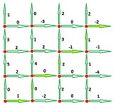
They are the inputs of the difference. Taken as a whole, the difference may look like this:

They are real-valued $1$-forms! Why aren't they vectors? They are if you take into account the direction of the corresponding edge. It is then a (real-valued) $1$-form, the difference of a $0$-form $f$. In fact, for an abbreviated notation, we combine the two differences into a single vector: $$\Delta f=\big<\Delta_x f,\Delta_y f\big>.$$

Example (hydraulic analogy). A simple interpretation of this data is water flow, as follows:

• each edge of the partition represents a pipe;
• $f(x_i,y_j)$ represents the water pressure at the joint $(x_i,y_j)$;
• the difference of the pressure between any two adjacent joints causes the water to flow;
• $\Delta_x f(s_{i},y_j)$ and $\Delta_y f(x_i,t_{j})$ are the flow amounts along these pipes; and
• $\frac{\Delta f}{\Delta x}(s_{i},y_j)$ and $\frac{\Delta f}{\Delta y}(x_i,t_{j})$ are the flow rates along these pipes.

For electric current, substitute “electric potential” for “pressure”. $\square$

According to our interpretation, only the flow along the pipe matters while any leakage is ignored. We can choose to take the latter into account and consider vector fields (or vector-valued $1$-forms); there is a vector assigned to each edge: $$\begin{array}{llllll} F(s,y)&=\big<&p(s,y) &,q(s,y)&\big>,\\ F(x,t)&=\big<&r(s,y)&,s(x,t)&\big>. \end{array}$$ In other words, there is also a component perpendicular to the corresponding edge:

However, only the projections of these vectors on the edges matter!

Definition. A vector field $F$ defined at each secondary node of the partition is called gradient if there is such a function $z=f(x,y)$ defined on the nodes of the partition that $$F(N)\cdot E=\Delta f\, (N),$$ for every edge $E$ and its secondary node $N$.

It follows that

• the horizontal component of $F(N)$ is equal to $\frac{\Delta f}{\Delta x}(N)$ when $N$ is on a horizontal edge, and
• the vertical component of $F(N)$ is equal to $\frac{\Delta f}{\Delta y}(N)$ when $N$ is a vertical edge.

The other components are irrelevant.

Example.

Next, we continue in the same manner as before: $$\lim_{\Delta X\to 0}\left( \begin{array}{cc}\text{ discrete }\\ \text{ calculus }\end{array} \right)= \text{ calculus }$$

The average and the instantaneous rates of change

Recall the $1$-dimensional case. A linear approximation of a function $y=f(x)$ at $x=a$ is function that defines a secant line, i.e., a line on the $xy$-plane through the point of interest $(a,f(a))$ and another point on the graph $(x,f(x))$. Its slope is the difference quotient of the function: $$\frac{\Delta f}{\Delta x}=\frac{f(x)-f(a)}{x-a}.$$

Now, let's see how this plan applies to functions of two variables. A linear approximation of a function $z=f(x,y)$ at $(x,y)=(a,b)$ is a function that represents a secant plane, i.e., a plane in the $xyz$-space through the point of interest $(a,b,f(a,b))$ and two other points on the graph. In order to ensure that these points define a plane, they should be chosen in such a way that they aren't on the same line. The easiest way to accomplish that is to choose the last two to lie in the $x$- and the $y$-directions from $(a,b)$, i.e., $(x,b)$ and $(a,y)$ with $x\ne a$ and $y\ne b$.

The two slopes in these two directions are the two difference quotients, with respect to $x$ and with respect to $y$: $$\frac{\Delta f}{\Delta x}=\frac{f(x,b)-f(a,b)}{x-a} \text{ and } \frac{\Delta f}{\Delta y}=\frac{f(a,y)-f(a,b)}{y-b}.$$

The two lines form the secant plane.

Definition. The partial derivatives of $f$ with respect to $x$ and $y$ at $(x,y)=(a,b)$ are defined to be the limits of the difference quotients with respect to $x$ at $x=a$ and with respect to $y$ at $y=b$ respectively, denoted by: $$\frac{\partial f}{\partial x}(a,b) = \lim_{x\to a}\frac{f(x,b)-f(a,b)}{x-a}\text{ and } \frac{\partial f}{\partial y}(a,b)= \lim_{y\to b}\frac{f(a,y)-f(a,b)}{y-b},$$ as well as $$f_x'(a,b)\text{ and } f'_y(a,b).$$

The following is an obvious conclusion.

Theorem. The partial derivatives of $f$ at $(x,y)=(a,b)$ are found as the derivatives of $f$ with respect to $x$ and to $y$: $$\frac{\partial f}{\partial x}(a,b) = \frac{d}{dx}f(x,b)\bigg|_{x=a},\ \frac{\partial f}{\partial y}(a,b)= \frac{d}{dy}f(a,y)\bigg|_{y=b}.$$

As a result, the computations are straight-forward.

Example. Find the partial derivatives of the function: $$f(x,y)=(x-y)e^{x+y^2}$$ at $(x,y)=(0,0)$: $$\begin{array}{ll} \frac{\partial f}{\partial x}(0,0) &= \frac{d}{dx}(x-0)e^{x+0^2}\bigg|_{x=0}&= \frac{d}{dx}xe^{x}\bigg|_{x=0}&=e^x+xe^x\bigg|_{x=0}&=1,\\ \frac{\partial f}{\partial y}(0,0) &= \frac{d}{dy}(0-y)e^{0+y^2}\bigg|_{y=0}&= \frac{d}{dy}-ye^{y^2}\bigg|_{y=0}&=-e^{y^2}-ye^{y^2}2y&=-e^{y^2}-2y^2e^{y^2}. \end{array}$$ $\square$

Example. Find the partial derivatives of the function: $$f(x,y)=$$ $\square$

Example. Now in reverse. Find a function $f$ of two variables the partial derivatives of which are these: $$\frac{\partial f}{\partial x}= ,\ \frac{\partial f}{\partial y}=$$ $\square$

Linear approximations and differentiability

This is the build-up for the introduction of the derivative of functions of two variables:

• the slopes of a surface in different directions,
• secant lines,
• secant planes,
• planes and ways to represent them, and finally
• limits.

Due to the complexity of the problem we will focus on the derivative at a single point for now.

Let's review what we know about the derivatives so far. The definition of the derivative of a parametric curve (at a point)is virtually identical to that for a numerical function because the fraction of the difference quotient is allowed by vector algebra: $$\begin{array}{cccc} &\text{numerical functions}\\ &f'(a)=\lim_{x\to a}\frac{f(x)-f(a)}{x-a}\\ \text{parametric curves} && \text{functions of several variables}\\ F'(a)=\lim_{t\to a}\frac{F(t)-F(a)}{t-a} && f'(A)=\lim_{X\to A}\frac{f(X)-f(A)}{X-A}\ ???\\ \end{array}$$ The same formula fails for a function of several variables. We can't divide by a vector! This failure is the reason why we start studying multi-dimensional calculus with parametric curves and not functions of several variables.

Can we fix the definition?

How about we divide by the magnitude of this vector? This is allowed by vector algebra and the result is something similar to the rise over the run definition of the slope.

Example. Let's carry out this idea for a linear function, the simplest kind of function: $$f(x,y)=2x+y.$$ The limit: $$\lim_{(x,y)\to (0,0)}\frac{|2x+y|}{\sqrt{x^2+y^2}},$$ is to be evaluated along either of the axes: $$\lim_{x\to 0}\frac{|2x+0|}{\sqrt{x^2+0^2}}=\lim_{x\to 0}\frac{|2x|}{|x|}=2\ \ne\ \lim_{y\to 0}\frac{|2\cdot 0+y|}{\sqrt{0^2+y^2}}=\lim_{y\to 0}\frac{|y|}{|y|}=1.$$ The limit doesn't exist because the slopes are different in different directions... $\square$

The line of attack of the meaning of the derivative then shifts -- to finding that tangent plane. Some of the functions shown in the last section have no tangent planes at their points of discontinuity. But such a plane is just a linear function! As such, it is a linear approximation of the function.

In the $1$-dimensional case, among the linear approximations of a function $y=f(x)$ at $x=a$ are the functions that define secant lines, i.e., lines on the $xy$-plane through the point of interest $(a,f(a))$ and another point on the graph $(x,f(x))$. Its slope is the difference quotient of the function: $$\frac{\Delta f}{\Delta x}=\frac{f(x)-f(a)}{x-a}.$$ In general, they are just linear functions and their graphs are lines through $(a,f(a))$; in the point-slope form they are: $$l(x)= f(a)+ m(x - a). $$ When you zoom in on the point, the tangent line -- but no other line -- will merge with the graph:

We reformulate our theory from Chapter 10 slightly.

Definition. Suppose $y=f(x)$ is a defined at $x=a$ and $$l(x)=f(a)+m(x-a)$$ is any of its linear approximations at that point. Then, $y=l(x)$ is called the best linear approximation of $f$ at $x=a$ if the following is satisfied: $$\lim_{x\to a} \frac{ f(x) -l(x) }{|x-a|}=0.$$

The definition is about the decline of the error of the approximation, i.e., the difference between the two functions: $$\text{error } = | f(x) -l(x) | . $$

This, not only the error vanishes, but also it vanishes relative to how close we are to the point of interest, i.e., the run. The following result is from Chapter 10.

Theorem. If $$l(x)=f(a)+m(x-a)$$ is the best linear approximation of $f$ at $x=a$, then $$m=f'(a).$$

Therefore, the graph of this function is the tangent line.

Now the partial derivatives of $f$ with respect to $x$ and $y$ at $(x,y)=(a,b)$ are: $$\frac{\partial f}{\partial x}(a,b) = \lim_{x\to a}\frac{f(x,b)-f(a,b)}{x-a}\text{ and } \frac{\partial f}{\partial y}(a,b)= \lim_{y\to b}\frac{f(a,y)-f(a,b)}{y-b}.$$

From our study of planes, we know that the vector formed by these functions that is especially important. It is called, again, the gradient and is defined to be (notation): $$\nabla f(a,b)=\bigg< \frac{\partial f}{\partial x}(a,b), \frac{\partial f}{\partial y}(a,b)\bigg>.$$

In general these approximations are just linear functions and their graphs are planes through the point $(a,b,f(a,b))$; in the point-slope form they are: $$l(x,y)= f(a,b)+ m(x - a)+n(y-b). $$ When you zoom in on the point, the tangent plane -- but no other plane -- will merge with the graph:

Definition. Suppose $y=f(x,y)$ is defined at $(x,y)=(a,b)$ function and $$l(x,y)=f(a,b)+m(x-a)+n(y-b)$$ is any of its linear approximations at that point. Then, $y=l(x,y)$ is called the best linear approximation of $f$ at $(x,y)=(a,b)$ if the following is satisfied: $$\lim_{(x,y)\to (a,b)} \frac{ f(x,y) -l(x,y) }{||(x,y)-(a,b)||}=0.$$ In that case, the function $f$ is called differentiable at $(a,b)$ and the graph of $z=l(x,y)$ is called the tangent plane.

In other words, we stick to the functions that look like plane on a small scale!

The definition is about the decline of the error of the approximation: $$\text{error } = | f(x,y) -l(x,y) | . $$ The limit of $\frac{\text{error}}{\text{run}}$ is required to be zero.

Theorem. If $$l(x,y)=f(a,b)+m(x-a)+n(y-b)$$ is the best linear approximation of $f$ at $x=a$, then $$m=\frac{\partial f}{\partial x}(a,b) \text{ and }n=\frac{\partial f}{\partial y}(a,b) .$$

Proof. The limit in the definition allows us to approach $(a,b)$ in any way we like. Let's start with the direction parallel to the $x$-axis and see how $\frac{\text{error}}{\text{run}}$ in converted into $\frac{\text{rise}}{\text{run}}$: $$\begin{array}{llcc} 0&=\lim_{x\to a^+,\ y=b} \frac{ f(x,y) -l(x,y) }{||(x,y)-(a,b)||}\\ &=\lim_{x\to a^+}\frac{ f(x,y) -(f(a,b) + m(x-a) +n(b-b))}{x-a}\\ &=\lim_{x\to a^+}\frac{ f(x,y) -f(a,b)}{x-a} -m \\ &= \frac{\partial f}{\partial x}(a,b) -m . \end{array}$$ The same computation for the $y$-axis produces the second identity. $\blacksquare$

Example. Let's confirm that the tangent plane to the hyperbolic paraboloid, given by the graph of $f(x,y)=xy$, at $(0,0)$ is horizontal: $$\frac{\partial f}{\partial x}(0,0)= \frac{d}{dx}f(x,0)\bigg|_{x=0}=\frac{d}{dx}(x\cdot 0)\bigg|_{x=0} =0,\ \frac{\partial f}{\partial y}(0,0)= \frac{d}{dy}f(0,y)\bigg|_{y=0}=\frac{d}{dx}(0\cdot y)\bigg|_{y=0} =0.$$

The two tangent lines form a cross and the tangent plane is spanned on this cross. $\square$

Just as before, replacing a function with its linear approximation is called linearization and it can be used to estimate values of new functions.

Example. Let's review a familiar example: approximation of $\sqrt{4.1}$. We can't compute $\sqrt{x}$ by hand because, in a sense, the function $f(x)=\sqrt{x}$ is unknown. The best linear approximation of $y=f(x)=\sqrt{x}$ is known and, as a linear function, it can be computed by hand: $$f'(x) = \frac{1}{2\sqrt{x}} \ \Longrightarrow\ f'(4) = \frac{1}{2\sqrt{4}} = \frac{1}{4}.$$ The best linear approximation is: $$l(x) = f(a) + f'(a) (x - a) = 2 + \frac{1}{4} (x - 4).$$ Finally, our approximation of $\sqrt{4.1}$ is $$l(4.1) = 2 + \frac{1}{4}(4.1 - 4) = 2 + \frac{1}{4} \cdot 1 = 2 + 0.025 = 2.025.$$

Let's now approximate of $\sqrt{4.1}\sqrt[3]{7.8}$. Instead of approximating the two terms separately, we will find the best linear approximation of the product $f(x,y)=\sqrt{x}\sqrt[3]{y}$ at $(x,y)=(4,8)$. Then we compute the partial derivatives, $x$: $$\frac{\partial f}{\partial x}(4,8)= \frac{d}{dx}f(x,8)\bigg|_{x=4}=\frac{d}{dx}\left(\sqrt{x}\sqrt[3]{8}\right)\bigg|_{x=4} =\frac{1}{2\sqrt{x}}2\bigg|_{x=4}=\frac{1}{2};$$ and $y$: $$\frac{\partial f}{\partial y}(4,8)= \frac{d}{dy}f(4,y)\bigg|_{y=8}=\frac{d}{dx}\left(\sqrt{4}\sqrt[3]{y}\right)\bigg|_{y=8} =2\frac{1/3}{\sqrt[3]{y^2}}\bigg|_{y=8}=\frac{1}{12}.$$ The best linear approximation is: $$l(x,y) = f(a,b) + \frac{\partial f}{\partial x}(a,b)(x - a) +\frac{\partial f}{\partial y}(a,b)(y-b)= 2\cdot 2 + \frac{1}{2} (x - 4)+\frac{1}{12} (y - 8).$$ Finally, our approximation of $\sqrt{4.1}\sqrt[3]{7.8}$ is $$l(4.1,7.8) = 4 + \frac{1}{2}.1+ \frac{1}{12}(-.2) = 4.033333....$$ $\square$

Exercise. Find the best linear approximation of $f(x)=(xy)^{1/3}$ at $(1,1)$.

To summarize,

• under the limit $x\to a$, the secant line parallel to the $x$-axis turns into a tangent line with the slope $f_x'(a,b)$, and
• under the limit $y\to b$, the secant line parallel to the $x$-axis turns into a tangent lines with the slope $f'_y(a,b)$,

provided $f$ is differentiable with respect to these two variables at this point. Meanwhile,

• the secant plane turns into the tangent plane,

provided $f$ is differentiable at this point, with the slopes $f_x'(a,b)$ and $f'_y(a,b)$ in the directions of the coordinate axes.

Partial differentiation and optimization

We pick one variable and treat the rest of them as parameters.

The rules are the same. This is, for example, the Constant Multiple Rule: $$\frac{\partial }{\partial x}(xy)=y\frac{\partial }{\partial x}(x)=...$$ This is the Sum Rule: $$\frac{\partial }{\partial x}(x+y)=y\frac{\partial }{\partial x}(x)=...$$

This notion is not to be confused with the “related rates”. Here $y$ is a function of $x$: $$\frac{d}{dx}\big( xy^2 \big)=y^2+x\cdot \frac{d}{dx}(y^2)=y^2+x\cdot 2yy',$$ by the Chain Rule. Here $y$ is just another variable: $$\frac{\partial}{\partial x}\big( xy^2 \big)=y^2+x\cdot \frac{\partial}{\partial x}(y^2)=y^2+x\cdot 0=y^2.$$ After all, these variable are un-related; they are independent variables!

Example. $\square$

Next we consider optimization, which is simply a way to find the maximum and minimum values of functions.

We already know from the Extreme Value Theorem that this problem always has a solution provided the function is continuous on a closed bounded subset.

Furthermore, just as in Chapter 9, we first narrow down our search. Recall that a function $y=f(x)$ has a local minimum point at $x = a$ if $f(a) \leq f(x)$ for all $x$ within some open interval centered at $a$. We can imagine as if we build a rectangle on top of each of these intervals and use to cut a piece from our graph.

We can't use intervals in dimension $2$, what's their analog? It is an open disk on the plane centered at $(a,b)$. We can imagine as if we build a cylinder on top of each of these disks and use to cut a patch from the surface of our graph.

In fact, both intervals and disks (and 3d balls, etc.) can be conveniently described in terms of the distance from the point: $d(X,A)\le \varepsilon$. So, we restrict our attention to these (possibly small) disks.

Definition. A function $z=f(X)$ has a local minimum point at $X = A$ if $f(A) \leq f(X)$ for all $X$ within some positive distance from $A$, i.e., $d(X,A)\le \varepsilon$. Furthermore, a function $f$ has a local maximum point at $X = A$ if $f(A) \geq f(X)$ for all $X$ for all $X$ within some positive distance from $A$. We call these local extreme points, or extrema.

Warning: The definition implies that $f$ is defined for all of these values of $X$.

Exercise. What could be a possible meaning of an analog of the one-sided derivative for functions of two variables?

In other words, there is an open disk $D$ around $A$ such that $A$ is the global maximum (or minimum) point when $f$ is restricted to $A$. Now, local extreme points are candidates for global extreme points. To compare to the familiar, one-dimensional case, we use to look at the terrain from the side and now we look from above:

How do we find them? We reduce the two-dimensional problem to the one-dimensional case. Indeed, if $(a,b)$ is a local maximum of $z=f(x,y)$ then

• $x=a$ is a local maximum of the numerical function $g(x)=f(x,b)$, and
• $y=b$ is a local maximum of the numerical function $h(y)=f(a,y)$.

In other words, the summit will be the highest point of our trip whether we come from the south or from the west.

Warning: with this approach we ignore the possibility of even higher locations found in the diagonal direction. However, the danger of missing this is only possible when the function isn't differentiable.

Just as in Chapter 9, we will use the derivatives in order to facilitate our search. Recall what Fermat’s Theorem states: if

• $x=a$ is a local extreme point of $z = f(x)$ and
• $z=f(x)$ is differentiable at $x=a$,

then $a$ is a critical point, i.e., $$f'(a)=0,$$ or undefined. The last equation typically produces just a finite number of candidates for extrema. As we apply the theorem to either variable, we find ourselves in a similar situation but with two equations.

File:Fermat’s Theorem dim 2.png

For a function of two variables we have the following two-dimensional analog of Fermat's Theorem.

Theorem (Fermat’s Theorem). If $X=A$ is a local extreme point of a differentiable at $A$ function several variables $z = f(X)$ then $A$ is a critical point, i.e., $$\nabla f \, (A)=0.$$

Example. Let's find the critical point of $$f(x,y)=x^2+3y^2+xy+7.$$ We differentiate: $$\begin{array}{lll} \frac{\partial f}{\partial x}(x,y)&=2x+y,\\ \frac{\partial f}{\partial x}(x,y)&=6y+x. \end{array}$$ We how set these derivatives equal to zero: $$\begin{array}{lll} 2x+y=0,\\ 6y+x=0. \end{array}$$ We have two equations to be solved. Geometrically, these are two lines and the solution is the intersection. By substitution: $$6y+x=0\ \Longrightarrow\ x=-6y\ \Longrightarrow\ 2(-6y)+y=0 \ \Longrightarrow\ y=0\ \Longrightarrow\ x=0.$$ There is only one critical point $(0,0)$. It is just a candidate for an extreme point, for now. Plotting reveals that this is a minimum. This is what the graph looks like:

This is a elliptic paraboloid (its level curves are ellipses). $\square$

Instead of one equation - one variable as in the case of a numerical function, we will have two variables - two equations (and then three variables - three equations, etc.). Typically the result is finitely many points.

Exercise. Give an example of a differentiable function of two variables with an infinitely many critical points.

Of course, the condition of the theorem -- partial derivatives are zero -- can be re-stated in a vector form -- the gradient is zero: $$f_x(a,b)=0 \text{ and } f_y(a,b)=0\ \Longleftrightarrow\ \nabla f(a,b)=0.$$ This means that the tangent plane is horizontal. So, at the top of the mountain, if it's smooth enough, it resembles a plane and this plane cannot be tilted because if it slopes down in any direction then so does the surface.

What we have seen is local optimization and it is only a stepping stone for global optimization. Just as in the one-dimensional case, the boundary points have to be dealt with separately. This time, however, there will be infinitely many of them instead of just two end-points:

Example. Let's find the extreme points of $$f(x,y)=x^2+y^2,$$ subject to the restriction (of the domain): $$|x|\le 1,\ |y|\le 1.$$ The restriction is the restriction of the domain of the function to this square.

We differentiate, set the derivatives equal to zero, and solve the system of equations: $$\begin{array}{lll} f_x(x,y)&=2x&=0&\Longrightarrow &x=0\\ f_y(x,y)&=2y&=0&\Longrightarrow &y=0 \end{array}\ \Longrightarrow\ (a,b)=(0,0).$$ This is the only critical point. We then note that $$f(0,0)=0$$ before proceeding.

The boundary points of our square domain remain to be investigated: $$|x|= 1,\ |y|= 1.$$ We have to test all of them by comparing the value of the function to each other and to the critical point. In other words, we are solving several one-dimensional optimization problems! These are the results: $$\begin{array}{lll} |x|=1&\Longrightarrow &f(x,y)=1+y^2&\Longrightarrow&\max_{|y|\le 1} \{1+y^2\}=2 \text{ for }y=\pm 1,&\min_{|y|\le 1} \{1+y^2\}=1 \text{ for }y=0,\\ |y|=1&\Longrightarrow &f(x,y)=x^2+1&\Longrightarrow&\max_{|x|\le 1} \{x^2+1\}=2 \text{ for }x=\pm 1,&\min_{|x|\le 1} \{x^2+1\}=1 \text{ for }x=0. \end{array}$$ Comparing these outputs we conclude that

• the maximal value of $2$ is attained at the four points $(1,1),(-1,1),(1,-1),(-1,-1)$, and
• the minimal value of $0$ is attained at $(0,0)$.

To confirm our conclusions we just look at the graph of this familiar paraboloid of revolution:

Under the domain restrictions, the graph doesn't look like a cup anymore... We can see the vertical parabolas we just maximized. $\square$

For functions of three variables, the domains are typically solids. The boundaries of these domains are then surfaces! Then, a part of such a 3d optimization problem will be a 2d optimization problem...

We can think of the pair of partial derivatives as one, the derivative, of a function of two variables. However, in sharp contrast to the one-variable case, the resulting function has a very different nature from the original: same input but the output isn't a number anymore but a vector! It's a vector field discussed in Chapter 19.

The second difference quotient with respect to a repeated variable

We start with numerical differentiation.

Example. We consider the function: $$f(x,y)=-x^2+y^2+xy.$$ When plotted, it is recognized as a familiar hyperbolic paraboloid.

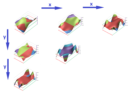
Below we outline the process of second partial differentiation. The variable functions -- with respect to $x$ and $y$ -- are shown and so are their derivatives. These are the functions we will differentiate.

First, for each value of $y$ given in the top row, we compute the difference quotient function with respect to $x$ by going down the corresponding column and then placing these values on right in a new table (it is one row short in comparison to the original): $$\texttt{=(RC[-29]-R[-1]C[-29])/R2C1}.$$

Second, for each value of $x$ given in the left-most column, we compute the difference quotient function with respect to $y$ by going right the corresponding row and then placing these values below in a new table (it is one column short in comparison to the original). $$\texttt{=(R[-29]C-R[-29]C[-1])/R2C1}.$$

This is the summary:

The two functions adjacent to the original are the familiar first partial derivatives. The top right and the bottom left are computed for the first time as described. The function in the middle is discussed in the next section.

The results are all horizontal lines equally spaced and in both cases they form horizontal planes. These planes are the graphs of the two new functions of two variables, the second partial derivatives, the tables of which have been constructed. Some things don't change: just as in the one-dimensional case, the second derivatives of quadratic functions are constant.

Here is a more complex example: $$f(x,y)=-x^2+y^2+xy+\sin(x+y+3).$$

$\square$

First, we notice that, just as with numerical functions in Chapter 8 and just as with the parametric curves in Chapter 17, the difference of the difference is simply the difference that skips a node. That's why the second difference doesn't provide us -- with respect to the same variable -- with any meaningful information. We will limit our attention to the difference quotients.

We will carry out the same second difference quotient construction for $f$ with respect to $x$ with $y$ fixed and then vice versa. The construction is summarized in this diagram: $$\begin{array}{ccc} -&f(x_1)&---&f(x_2)&---&f(x_3)&-&\\ -&-\bullet-&\frac{\Delta f}{\Delta x_2}&-\bullet-&\frac{\Delta f}{\Delta x_3}&-\bullet-&-\\ -&-\bullet-&---&\frac{\frac{\Delta f}{\Delta x_3} -\frac{\Delta f}{\Delta x_2}}{s_3-s_2}&---&-\bullet-&-&\\ &x_1&s_2&x_2&s_3&x_3&\\ \end{array}$$

The two computations are illustrated by continuing the following familiar diagram for the (first) partial difference quotients: $$\begin{array}{ccccccc} f(x,y+\Delta y)&---&f(x+\Delta x,y+\Delta y)&&-\bullet-&\frac{\Delta f}{\Delta x} f(s,y+\Delta y)&-\bullet-\\\\ |&&|&&|&&|\\ |&&|&\leadsto&\frac{\Delta f}{\Delta y}(x,t)&&\frac{\Delta f}{\Delta y}(x+\Delta x,t)\\ |&&|&&|&&|\\ f(x,y)&---&f(x+\Delta x,y)&&-\bullet-&\frac{\Delta f}{\Delta x}(s,y)&-\bullet- \end{array}\leadsto$$ There are two further diagrams. We, respectively, subtract the numbers assigned to the horizontal edges horizontally (shown below) and we subtract the numbers assigned to the vertical edges vertically before placing the results at the nodes (not shown): $$\begin{array}{ccc} -\bullet-&\frac{\Delta f}{\Delta x}(s,y)&-\bullet-&\frac{\Delta f}{\Delta x}(s+\Delta s,y)&-\bullet- \end{array}\quad\leadsto\quad\begin{array}{ccc} -\bullet-&--&\frac{\Delta \frac{\Delta f}{\Delta x}}{\Delta x}(x,y)&--&-\bullet- \end{array}$$

Recall from earlier in this chapter that we have a partition $P$ of a rectangle $R=[a,b]\times [c,d]$ in the $xy$-plane built as a combination of partitions of the intervals $[a,b]$ and $[c,d]$: $$a=x_{0}\le x_{1}\le x_{2}\le ... \le x_{n-1}\le x_{n}=b,$$ and $$c=y_{0}\le y_{1}\le y_{2}\le ...\le y_{m-1}\le y_{m}=d.$$ Its primary nodes are: $$X_{ij}=(x_i,y_{j}),\ i=1,2,...,n,\ j=1,2,...,m;$$ and its secondary nodes are:

• a point $S_{ij}$ in the segment $[x_{i-1},x_{i}]\times \{y_{j}\}$, and
• a point $T_{ij}$ in the segment $\{x_{i}\}\times [y_{j-1},y_{j}]$.

If $z=f(x,y)$ is defined at the nodes $X_{ij},\ i,j=0,1,2,...,n$, of the partition, the partial difference quotients of $f$ with respect to $x$ and $y$ are respectively: $$\frac{\Delta f}{\Delta x}(S_{ij})=\frac{f(X_{ij})-f(X_{i-1,j})}{x_{i}-x_{i-1}}\text{ and }\frac{\Delta f}{\Delta y}(T_{ij})=\frac{f(X_{ij})-f(X_{i,j-1})}{y_{j}- y_{j-1}}.$$

It is now especially important that we have utilized the secondary nodes as the inputs of the new functions. Indeed, we can now carry out a similar construction with these functions and find their difference quotients, the four of them. The construction is based on the one we carried out for functions of one variable in Chapter 7:

We will start with these two new quantities.

First, let's consider the rate of change of $\frac{\Delta f}{\Delta x}$ -- the rate of change of $f$ with respect to $x$ -- with respect to $x$, again. For each fixed $j$, we consider the partition of the horizontal interval $[a,b]\times \{y_{j}\}$ with the primary nodes: $$S_{ij}=(s_{ij},y_{j}),\ i=1,2,...,n,$$ and the secondary nodes: $$X_{ij},\ i=1,2,...,n-1.$$ We now carry out the same difference quotient construction, still within the horizontal edges.

Similarly, to define the rate of change of $\frac{\Delta f}{\Delta y}$ with respect to $y$. For each fixed $i$, we consider the partition of the vertical interval $\{x_{i}\}\times [c,d]$ with the primary nodes: $$T_{ij}=(x_{i},t_{ij}),\ j=1,2,...,m,$$ and the secondary nodes: $$X_{ij},\ j=1,2,...,m-1.$$ We now carry out the same difference quotient construction, still within the vertical edges.

Definition. The (repeated) second difference quotient of $f$ with respect to $x$ is defined at the primary nodes of the original partition $P$ by ($i=1,2,...,n-1,\ j=0,1,...,m$): $$\frac{\Delta^2 f}{\Delta x^2}(X_{ij})=\frac{\frac{\Delta f}{\Delta x}(S_{ij})-\frac{\Delta f}{\Delta x}(S_{i,j-1})}{s_{ij}-s_{i-1,j}} ;$$ and the second difference quotient of $f$ with respect to $y$ is defined at the primary nodes of the original partition $P$ by ($i=0,1,...,n,\ j=1,2,...,m-1$): $$\frac{\Delta^2 f}{\Delta y^2}(X_{ij})=\frac{\frac{\Delta f}{\Delta y}(T_{ij})-\frac{\Delta f}{\Delta y}(T_{i,j-1})}{t_{ij}-t_{i,j-1}}.$$

These are discrete $0$-forms.

In the above example, we can see how the sign of these expressions reveal the concavity of the curves.

For a simplified notation, we will often omit the indices: $$\frac{\Delta^2 f}{\Delta x^2}(x,y)=\frac{\frac{\Delta f}{\Delta x}(s+\Delta s,y)-\frac{\Delta f}{\Delta x}(s,y)}{\Delta s} ;$$ $$\frac{\Delta^2 f}{\Delta y^2}(x,y)=\frac{\frac{\Delta f}{\Delta y}(x,t+\Delta t)-\frac{\Delta f}{\Delta y}(x,t)}{\Delta t}.$$

Example.

The second difference and the difference quotient with respect to mixed variables

Furthermore, we can compute the rate of change of with respect to the other variable. This is how the concavity with respect to $x$ is increasing with increasing $y$:

We are not in the $1$-dimensional setting anymore! That is why, in contrast to the one-dimensional case in Chapter 7, the case of parametric curves in Chapter 17, and the repeated variable case above, the difference of the difference is not simply the difference that skips a node. The second difference with respect to mixed variables does provide us with meaningful information.

The partial differences: $$\Delta_x f\, (S_{ij}) \text{ and } \Delta_y f\, (T_{ij}),$$ and the partial difference quotients: $$\frac{\Delta f}{\Delta x}(S_{ij}) \text{ and } \frac{\Delta f}{\Delta y}(T_{ij}).$$ are defined at the secondary nodes located on the edges of the partition of the rectangle $[a,b]\times [c,d]$, horizontal and vertical:

There are four more quantities:

• the change of $\Delta_x f$ with respect to $y$,
• the change of $\Delta_y f$ with respect to $x$,
• the rate of change of $\frac{\Delta f}{\Delta x}$ with respect to $y$, and
• the rate of change of $\frac{\Delta f}{\Delta y}$ with respect to $x$.

They will be assigned to the nodes located at the faces of the original partition. These are tertiary nodes.

The new computations are illustrated by continuing the following familiar diagram for the (first) differences: $$\begin{array}{ccccccc} f(x,y+\Delta y)&---&f(x+\Delta x,y+\Delta y)&&-\bullet-&\Delta_x f\, (s,y+\Delta y)&-\bullet-\\ |&&|&&|&&|\\ |&&|&\leadsto&\Delta_y f\, (x,t)&&\Delta_y f\, (x+\Delta x,t)\\ |&&|&&|&&|\\ f(x,y)&---&f(x+\Delta x,y)&&-\bullet-&\Delta_x f\, (s,y)&-\bullet- \end{array}\leadsto$$ There are two further diagrams. We, respectively, subtract the numbers assigned to the horizontal edges vertically and we subtract the numbers assigned to the vertical edges horizontally before placing the results in the middle of the square: $$\leadsto\begin{array}{ccc} -\bullet-&---&-\bullet-\\ |&\Delta_y\Delta_x f\, (s,t)&|\\ -\bullet-&---&-\bullet- \end{array}\qquad\qquad \qquad\leadsto \begin{array}{ccc} -\bullet-&---&-\bullet-\\ |&\Delta_x\Delta_y f\, (s,t)&|\\ -\bullet-&---&-\bullet- \end{array}$$

Definition. The (mixed) second difference of $f$ with respect to $yx$ is defined at the tertiary nodes of the original partition $P$ by ($i=1,2,...,n-1,\ j=1,2,...,m-1$): $$\Delta^2_{yx} f\, (U_{ij})=\Delta_x f\, (S_{ij})-\Delta_x f\, (S_{i,j-1});$$ and the mixed difference quotient of $f$ with respect to $xy$ is defined at the tertiary nodes of the original partition $P$ by ($i=1,2,...,n-1,\ j=1,2,...,m-1$): $$\Delta^2_{xy} f\, (U_{ij})=\Delta_y f\, (T_{ij})-\Delta_y f\, (T_{i-1,j}).$$

Definition. The (mixed) second difference quotient of $f$ with respect to $yx$ is defined at the tertiary nodes of the original partition $P$ by ($i=1,2,...,n-1,\ j=1,2,...,m-1$): $$\frac{\Delta^2 f}{\Delta y \Delta x}(U_{ij})=\frac{\frac{\Delta f}{\Delta x}(S_{ij})-\frac{\Delta f}{\Delta x}(S_{i,j-1})}{y_{j}-y_{j-1}};$$ and the mixed difference quotient of $f$ with respect to $xy$ is defined at the tertiary nodes of the original partition $P$ by ($i=1,2,...,n-1,\ j=1,2,...,m-1$): $$\frac{\Delta^2 f}{\Delta x \Delta y}(U_{ij})=\frac{\frac{\Delta f}{\Delta y}(T_{i,j})-\frac{\Delta f}{\Delta y}(T_{i-1,j})}{x_{i}-x_{i-1}}.$$

When the tertiary nodes are unspecified, these are functions of the faces themselves, i.e., discrete $2$-forms.

For a simplified notation, we will often omit the indices: $$\frac{\Delta^2 f}{\Delta y \Delta x}(s,t)=\frac{\frac{\Delta f}{\Delta x}(s,y+\Delta y)-\frac{\Delta f}{\Delta x}(s,y)}{\Delta y};$$ $$\frac{\Delta^2 f}{\Delta x \Delta y}(s,t)=\frac{\frac{\Delta f}{\Delta y}(x+\Delta x,t)-\frac{\Delta f}{\Delta y}(x,t)}{\Delta x}.$$

Now, the two mixed differences are “made of” the same four quantities; one can guess that they are equal. For example, we can see it here:

Let's confirm that with algebra. We substitute and simplify: $$\begin{array}{lll} \Delta_{yx}^2 f\, (s,t)&=\Delta_x f\, (s,y+\Delta y)-\Delta_x f\, (s,y)\\ &=\big( f(x+\Delta x,y+\Delta y)-f(x,y+\Delta y)\big)-\big(f(x+\Delta x,y)-f(x,y)\big)\\ &=f(x+\Delta x,y+\Delta y)-f(x,y+\Delta y)-f(x+\Delta x,y)+f(x,y)\\ &=\big(f(x+\Delta x,y+\Delta y)-f(x+\Delta x,y)\big)-\big( f(x,y+\Delta y)-f(x,y)\big)\\ &=\Delta_y f\, (x+\Delta x,t)-\Delta_y f\, (x,t)\\ &=\Delta_{xy}^2 f\, (s,t). \end{array}$$

Theorem (Discrete Clairaut's Theorem). Over a partition in ${\bf R}^n$, first, the mixed second differences with respect to any two variables are equal to each other: $$\Delta_{yx}^2 f=\Delta_{xy}^2 f;$$ and, second, the mixed second difference quotients are equal to each other: $$\frac{\Delta^2 f}{\Delta y \Delta x}=\frac{\Delta^2 f}{\Delta x \Delta y}.$$

This theorem will have important consequences presented in Chapter 19.

The second partial derivatives

The second derivative is known to help to classify extreme points. At least, we can dismiss the possibility that a point is a maximum when the function is concave up, i.e., the second derivative is positive.

Example. In the above example of the function $$f(x,y)=x^2+3y^2+xy+7,$$ we differentiate one more time each partial derivative -- with respect to the same variable: $$\begin{array}{lll} \frac{\partial f}{\partial x}&=2x+y&\Longrightarrow&\frac{\partial }{\partial x}\left( \frac{\partial f}{\partial x}\right)&=\frac{\partial }{\partial x}(2x+y)&=2,\\ \frac{\partial f}{\partial x}&=6y+x&\Longrightarrow&\frac{\partial }{\partial y}\left( \frac{\partial f}{\partial y}\right)&=\frac{\partial }{\partial x}(6y+x)&=6. \end{array}$$ Both numbers are positive, therefore, both curves are concave up! $\square$

Repeated differentiation produces a sequence of functions in the one variable case: $$\newcommand{\ra}[1]{\!\!\!\!\!\xrightarrow{\quad#1\quad}\!\!\!\!\!} \newcommand{\la}[1]{\!\!\!\!\!\xleftarrow{\quad#1\quad}\!\!\!\!\!} \newcommand{\da}[1]{\left\downarrow{\scriptstyle#1}\vphantom{\displaystyle\int_0^1}\right.} \newcommand{\ua}[1]{\left\uparrow{\scriptstyle#1}\vphantom{\displaystyle\int_0^1}\right.}\begin{array}{cccccccccccc} f &\ra{\frac{d}{dx}} &f' &\ra{\frac{d}{dx}} & f' ' &\ra{\frac{d}{dx}} &...&\ra{\frac{d}{dx}} & f^{(n)} &\ra{\frac{d}{dx}} & ... \end{array}$$ In the two-variable case, it makes the functions multiply: $$\begin{array}{cccccccccccc} &&&& &f\\ &&&&\swarrow_x&&_y\searrow\\ &&&f_x& && &f_y\\ &&\swarrow_x&&_y\searrow&&\swarrow_x&&_y\searrow\\ &f_{xx}&&&&f_{yx}\quad f_{xy}&&&&f_{yy}\\ \swarrow_x&&_y\searrow&&\swarrow_x&&_y\searrow&&\swarrow_x&&_y\searrow\\ ...&&...&&...&&...&&...&&... \end{array}$$

The number of derivatives might be reduced when the mixed derivatives at the bottom are equal. It is often possible thanks to the following result that we accept without proof.

Theorem (Clairaut's theorem). Suppose a function $z=f(x,y)$ has continuous second partial derivatives at a given point $(x_0,y_0)$ in ${\bf R}^2$. Then we have: $$\frac{\partial^2 f}{\partial x\, \partial y}(x_0,y_0) = \frac{\partial^2 f}{\partial y\, \partial x}(x_0,y_0).\,$$

Under the conditions of the theorem, this part of the above diagram becomes commutative: $$\begin{array}{cccccccccccc} &&&& &f\\ &&&&\swarrow_x&&_y\searrow\\ &&&f_x& && &f_y\\ &&\swarrow_x&&_y\searrow&&\swarrow_x&&_y\searrow\\ &f_{xx}&&&&f_{yx}= f_{xy}&&&&f_{yy}\\ \end{array}$$ In fact, the two operations of partial differentiation commute: $$\frac{\partial}{\partial x}\frac{\partial}{\partial y}=\frac{\partial}{\partial y}\frac{\partial}{\partial x}.$$ This can also be written as another commutative diagram: $$\newcommand{\ra}[1]{\!\!\!\!\!\!\!\xrightarrow{\quad#1\quad}\!\!\!\!\!} \newcommand{\da}[1]{\left\downarrow{\scriptstyle#1}\vphantom{\displaystyle\int_0^1}\right.} % \begin{array}{llr} f & \ra{\frac{\partial}{\partial x}} & f_x \\ \da{\frac{\partial}{\partial y}} & \searrow & \da{\frac{\partial}{\partial y}} \\ f_y & \ra{\frac{\partial}{\partial x}} & f_{xy}=f_{yx} \end{array}$$

For the case of three variables, there are even more derivatives: $$\begin{array}{cccccccccccc} &&&& &&&f\\ &&&&\swarrow_x&&&\downarrow_y&&&_z\searrow\\ &&&f_x& && &f_y& && &f_z\\ &&\swarrow_x&\downarrow_y&_z\searrow&&\swarrow_x&\downarrow_y&_z\searrow&&\swarrow_x&\downarrow_y&_z\searrow\\ &f_{xx}&&f_{yx}&&f_{zx}\quad f_{xy}&&f_{yy}&&f_{zy}\quad f_{xz}&&f_{xz}&&f_{yz}\ f_{zz}\\ \end{array}$$ Under the conditions of the theorem, the three operations of partial differentiation commute (pairwise): $$\frac{\partial}{\partial x}\frac{\partial}{\partial y}=\frac{\partial}{\partial y}\frac{\partial}{\partial x},\ \frac{\partial}{\partial y}\frac{\partial}{\partial z}=\frac{\partial}{\partial z}\frac{\partial}{\partial y},\ \frac{\partial}{\partial z}\frac{\partial}{\partial x}=\frac{\partial}{\partial x}\frac{\partial}{\partial z}.$$ The above diagram also becomes commutative: $$\newcommand{\ra}[1]{\!\!\!\!\!\!\!\xrightarrow{\quad#1\quad}\!\!\!\!\!} \newcommand{\la}[1]{\!\!\!\!\!\!\!\xleftarrow{\quad#1\quad}\!\!\!\!\!} % \begin{array}{cccccccccccc} &&&& &f_{zz}\\ &&&& &\uparrow_z\\ &&&\la{}& \la{} &f_z& \ra{} & \ra{}\\ && \swarrow^x& &&\uparrow_z&&&^y\searrow\\ &&f_{xz}=&f_{zx}& & f && f_{zy}&=f_{yz}\\ &&&\uparrow_z&\swarrow^x&&^y\searrow&\uparrow_z\\ &&&f_x& && &f_y\\ &&\swarrow^x&&^y\searrow&&\swarrow^x&&^y\searrow\\ &f_{xx}&&&&f_{yx}= f_{xy}&&&&f_{yy}\\ \end{array}$$