Applications of ODEs

Pursuit curves

In this chapter, we will often refer to systems of ODEs as vector ODEs or simply ODEs.

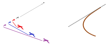
Imagine a hound running after a rabbit. Let's investigate their mutual dynamics.

We assume that the hound is always heading at the rabbit while the rabbit is heading for its hole and never changes directions.

We build a discrete model. This means that the time progresses in increments: $$t_0=0,\ t_{n+1}=t_n+\Delta t.$$ The main assumption is:

• during the time interval $[t_n,t_n+\Delta t]$, the hound will be running toward the spot where the rabbit was at time $t_n$.

Suppose their locations are:

• $(x,y)$ is the location of the rabbit, and
• $(p,q)$ is the location of the hound.

They are represented by parametric curves defined at the nodes of the standard partition of the real line:

• $(x_n,y_n)=(x(t_n),y(t_n))$ is the location of the rabbit after $n$ increments, and
• $(p_n,q_n)=(p(t_n),q(t_n))$ is the location of the hound after $n$ increments.

On the left we have, just as before, a simplified notation.

Suppose

• $s$ is the speed of the rabbit, and
• $v$ is the speed of the hound, $v>s$.

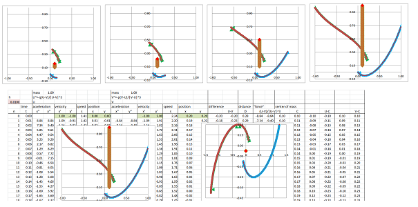
Example. We create a model for the hound that is independent of a specific choice of the path of the rabbit: one step at a time.

We compute consecutively:

• the difference between the two: $x_n-p_n$ and $y_n-q_n$, which is the direction from the hound towards the rabbit;
• the unit vector in this direction (dividing by the distance between them);
• the velocity of the hound (multiplying this vector by the hounds' speed $v$); and
• the new location $(p_{n+1},q_{n+1})$ of the hound (adding the velocity times time interval $h=\Delta t$ to the last location).

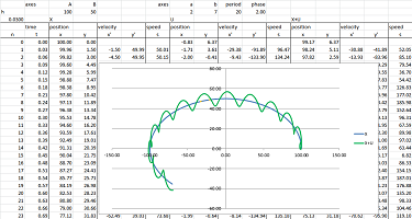
Above and below left is the pursuit of a rabbit following a circular path. Below right is a sinusoid:

$\square$

Exercise. Implement this model for the case of the rabbit running north-west:

Exercise. Implement this model for the case of the rabbit following a circle, sinusoid, spiral, etc.

We now approach this analytically. To make this possible, we choose a simple case: the rabbit is running along the $y$-axis from the origin. Then, $$\begin{cases} x_{n+1}=0,\\ y_{n+1}=y_n+s\Delta t. \end{cases}$$ Furthermore,

• $\Delta x_n=\Delta x\, (c_n)$,
• $\Delta y_n=\Delta y\, (c_n)$,
• $\Delta p_n=\Delta p\, (c_n)$,
• $\Delta q_n=\Delta q\, (c_n)$,

where $c_n$ are, say, the mid-points of the intervals of the partition. For the hound, we have: $$\begin{cases} p_{n+1}=p_n+\Delta p_n,\\ q_{n+1}=q_n+\Delta q_n. \end{cases}$$ We assume that the hound is located to the right of the $y$-axis and, therefore, moving to its left, $\Delta x_n<0$. As the hound moves from $(p_n,q_n)$ in the direction of $(x_n,y_n)$, the two right triangles are similar:

• first, the one with the sides $p_n-x_n$ and $y_n-q_n$, and
• second, the one with the sides $-\Delta p_n$ and $\Delta q_n$.

These observations give us the discrete model for the hound. We have for the tangent of the base angle of these triangles: $$\tau_n=\frac{y_n-q_n}{p_n-x_n}=\frac{\Delta q_n}{-\Delta p_n}.$$ Therefore, we have a recursive formula for $\Delta q_n$, $$\Delta q_n=-\tau_n\cdot \Delta p_n,$$ if we can just find $\Delta p_n$. The hypotenuse of the latter triangle is $$(\Delta p_n)^2+(\Delta q_n)^2=(v\cdot \Delta t)^2.$$ We derive from the last equation the following: $$1+\tau_n^2=1+\left(\frac{\Delta q_n}{\Delta p_n}\right)^2=\left(\frac{v\cdot \Delta t}{\Delta p_n}\right)^2.$$ Solving this equation for $\Delta p_n$, we choose the negative sign for the square root: $$\Delta p_n=-\frac{v}{\sqrt{1+\tau_n^2}}\Delta t.$$

Warning: If the rabbit gets to the right of the hound, one has to change the sign.

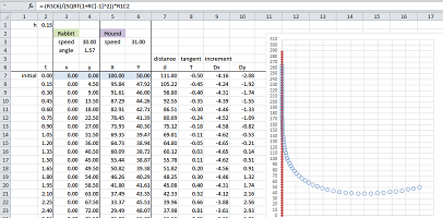
Example. Let's confirm our analysis with a spreadsheet. The setting are the following:

• $\Delta t=.1$ seconds,
• $s=30$ feet per second;
• $v=31$ feet per second;
• $(x_0,y_0)=(0,0)$ feet,
• $(p_0,q_0)=(100,50)$ feet.

The main formulas are the ones for $\Delta p_n$ and $\Delta q_n$: $$\texttt{=-(R3C6)/(SQRT(1+RC[-1]^2))*R1C2},\quad \texttt{=-RC[-2]*RC[-1]}.$$ The results match those acquired via a discrete model. $\square$

From the two recursive formulas, we derive via substitution: $$\begin{array}{lll} \Delta p_n=-\frac{v}{\sqrt{1+\tau_n^2}}\Delta t,&\Longrightarrow&\frac{\Delta p_n}{\Delta t}=-\frac{v}{\sqrt{1+\tau_n^2}},\\ \Delta q_n=-\tau_n\cdot \Delta p_n,&\Longrightarrow&\frac{\Delta q_n}{\Delta t}=\frac{v\tau_n}{\sqrt{1+\tau_n^2}}. \end{array}$$

Then, via $\Delta t\to 0$, we arrive at two time-dependent ODEs: $$\begin{cases} \frac{d p}{d t}=-\frac{v}{\sqrt{1+\tau^2}},\\ \frac{d q}{d t}=\frac{v\tau}{\sqrt{1+\tau^2}}, \end{cases}$$ where $$\tau=\frac{y-q}{p-x},$$ and $(x,y)$ is the fixed parametric curve representing the motion of the rabbit.

Now, let's see what this analysis looks like in the vector notation. Suppose, as before, $H$ is the location of the hound and $R$ is the location of the rabbit. The latter is known. For the former, the displacement vector $\Delta H$ of $H$ has to be collinear to the vector from $H$ to $R$.

Therefore, $$\Delta H \cdot HR=||\Delta H||\cdot ||HR||=S||HR||.$$ The formula applies to any mutual location of the rabbit and the hound as well to pursuits in a space of any dimension.

Exercise. Derive an explicit ODEs for the case when the rabbit follows a straight path.

ODEs of second order as systems

We previously discussed how ODEs of second order model motion of objects affected by forces. A special case is a linear ODE: $$\frac{\Delta^2 x}{\Delta t^2}= a\frac{\Delta x}{\Delta t}+bx \text{ and }x' '=ax'+bx.$$ Here,

• $x$ is the position,
• $\frac{\Delta x}{\Delta t}$ and $x'$ is the velocity,
• $\frac{\Delta^2 x}{\Delta t^2}$ and $x' '$ is the acceleration.

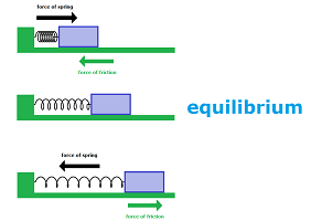
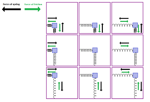
Meanwhile $a$ and $b$ are constant numbers that express the proportional dependence of the force (i.e., the acceleration) on the velocity and the position respectively. For example, the object may be attached to the wall by a spring and, at the same time, be affected by the friction of the surface.

In fact, it makes sense to assume the following:

• the spring has its Hooke's force proportional to the displacement from the equilibrium, with coefficient $b$, and since it pulls in the direction opposite to the displacement, we conclude that $b\le 0$; and
• the friction force is proportional to the velocity, with coefficient $a$, and since it pulls in the direction opposite to the velocity, we conclude that $a\le 0$.

These will be our assumptions: $$a\le 0,\ b< 0.$$

In chapter 21 we used the discrete equation above to the motion of spring and other dynamics. What about the other equation? In the simplest case $a=0$, it was also solved. In our attempt to solve this equation in the general case we realize that we have no methods developed for equations of second order! When we encounter a completely new situation, we should always try to reduce it to something familiar.

We will apply the following clever trick. We introduce an extra (dependent) variable: $$y=x'.$$ In terms of motion, the trick is nothing but re-introducing the velocity back into the picture. The result is a system of two ODEs: $$\begin{cases} x'&=&&y,\\ y'&=bx&+&ay. \end{cases}$$ The result is a trade-off: increasing the dimension -- from $1$ to $2$ -- but decreasing the order -- from $2$ for $1$ -- of the system. This $2\times 2$ linear vector ODE, $$X'=FX, \text{ with } F=\left[\begin{array}{cc} 0&1\\ b&a \end{array}\right],$$ can now be subjected to the classification analysis presented in the last chapter.

First, the characteristic polynomial is: $$\chi(\lambda)=\lambda^2 -a\lambda - b.$$ Suppose $\lambda_1$ and $\lambda_2$ are its two roots: $$\lambda_{1,2}=\frac{a}{2}\pm\frac{\sqrt{a^2+4b}}{2}.$$ Then the outcomes depend on the sign of the discriminant, $$D=a^2+4b.$$ Consider the case of $D\ge 0$. Since $a\le 0$, we have $$\lambda_{1}= \frac{a}{2}-\frac{\sqrt{a^2+4b}}{2}< 0.$$ Since $b< 0$, we conclude that $$\lambda_{1}= \frac{a}{2}+\frac{\sqrt{a^2+4b}}{2}<\frac{a}{2}+\frac{\sqrt{a^2}}{2}=\frac{a}{2}+\frac{-a}{2}=0$$ Therefore, an important conclusion is that the real eigenvalues are always negative.

According to our classification theorem, there are three main cases:

• Case #1: two distinct real roots;
• Case #2: one real repeated root;
• Case #3: complex conjugate roots.

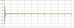
Case #1 is the case of $$D=a^2+4b>0.$$ The general solution is given by $$x = C e^{\lambda_{1}t} + K e^{\lambda_2t}. $$ As $\lambda_{1},\lambda_2<0$, we have exponential decay (a stable node of the vector ODE): the friction brings the ODE back to the equilibrium without oscillating. Here Euler's method is run with $a=-8,\ b=-1$:

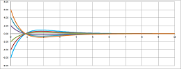
Case #2 is the case of $$D=a^2+4b=0.$$ Again, as $\lambda=\lambda_{1}=\lambda_2<0$, we see exponential decay (a stable improper node of the ODE): the ODE's motion dies out, even though it might overshoot. The general solution is given by $$x = ( C + K t ) e^{\lambda t}.$$ Here Euler's method is run with $a=-2,\ b=-1$:

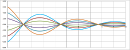
Case #3 is the case of $$D=a^2+4b<0.$$ The general solution is given by $$x = C e^{\alpha t} \cos(\beta t) + K e^{\alpha t} \sin(\beta t),$$ where $$\alpha=\operatorname{Re}\lambda_{1,2}=\frac{a}{2}$$ is non-negative by assumption and $$\beta=\operatorname{Im}\lambda_{1,2}=\pm\frac{\sqrt{D}}{2}$$ is non-zero because $D\ne 0$. When $a<0$, we see an oscillating decay (a stable focus of the ODE): the friction is strong enough to bring the ODE to the equilibrium eventually but isn't strong enough to stop the ODE from oscillating. Here Euler's method is run with $a=-.5,\ b=-1$:

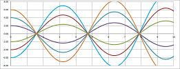
When $a=0$, we see pure oscillation (a center of the ODE): no friction. Here Euler's method is run with $a=0,\ b=-1$:

Looking at these illustration as a sequence reveals the effect of growing of the friction coefficient $b$.

Exercise. Point out in what way the last illustration doesn't match the description and explain why.

Vector ODEs of second order: a double spring

What of the nature of the forces remains the same but the motion is on the plane?

In the simplest situation,

• two different springs are attached to the object along the two axes;
• two different kinds of friction are produced along the two axes.

As the object moves,

• two springs exert two forces along the axes -- negatively proportional to the displacement from the equilibrium;
• two kinds of friction exert two forces along the axes -- negatively proportional to the velocity.

The displacements and the velocities of the object in the two directions are independent of each other. Therefore, there will be two linear ODE of order $2$ of the same kinds as before: $$x' '=ax'+bx \text{ and } y' '=cy'+dy ,$$ where $$a\le 0 \text{ and }b\le 0 \text{ and } c\le 0 \text{ and }d\le 0.$$ In this case, the classification in the last section applies, separately. We combine the two scalar equations into one vector equation: $$\begin{cases} x' '&=ax'&+bx \\ y' '&=cy'&+dy \end{cases}\quad\leadsto\quad \left[\begin{array}{cc}x' '\\ y' '\end{array}\right]=\left[\begin{array}{cc}a&0\\ 0&c\end{array}\right] \left[\begin{array}{cc}x'\\ y'\end{array}\right]+\left[\begin{array}{cc}b&0\\ 0&d\end{array}\right]\left[\begin{array}{cc}x \\ y\end{array}\right] $$

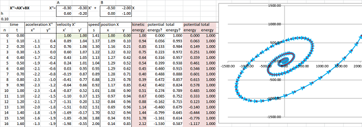
Generally, we have a vector ODE: $$X' '=AX'+BX.$$ Here, $$X=\left[\begin{array}{cc}x \\ y\end{array}\right],\quad X'=\left[\begin{array}{cc}x'\\ y'\end{array}\right],\quad X' '=\left[\begin{array}{cc}x' '\\ y' '\end{array}\right]$$ are the position vector, the velocity, and the acceleration, respectively. Also, $A$ and $B$ are two $2\times 2$ matrices that express the (linear) dependence of the force (i.e., the acceleration) on the velocity and position respectively. They don't have to be diagonal anymore.

In contrast to the last section, we will concentrate on the discrete ODEs: $$\frac{\Delta^2 X}{\Delta t^2}=A\frac{\Delta X}{\Delta t}+BX.$$ Here, a solution $X$ is a parametric curve defined on the nodes of a partition of an interval, $t_0,t_1,...$ (i.e., a discrete $0$-form), so that its difference quotient and the second difference quotient satisfy the equation: $$X=\left[\begin{array}{cc}x \\ y\end{array}\right],\quad \frac{\Delta X}{\Delta t}=\left[\begin{array}{cc}\frac{\Delta x}{\Delta t}\\ \frac{\Delta y}{\Delta t}\end{array}\right],\quad \frac{\Delta^2 X}{\Delta t^2}=\left[\begin{array}{cc}\frac{\Delta^2 x}{\Delta t^2}\\ \frac{\Delta^2 y}{\Delta t^2}\end{array}\right].$$

In order to simplify the notation, we define three sequences of vectors in ${\bf R}^2$: $$\begin{array}{lll} X_{n}' '=\frac{\Delta^2 X}{\Delta t^2}(t_n);\\ X_{n}'=\frac{\Delta X}{\Delta t}(t_n);\\ X_{n}=X_(t_n). \end{array}$$ The ODE then produces these three recursive formulas for those three sequences of vectors: $$\begin{array}{lll} X_{n+1}' '=AX_n'+BX_n;\\ X_{n+1}'=X_n'+X_{n+1}' '\, \Delta t;\\ X_{n+1}=X_n+X_{n+1}'\, \Delta t. \end{array}$$ We apply them below.

The starting point is the simplest case of the two springs. Here, the matrices are diagonal: $$A=\left[\begin{array}{rr} a_x&0 \\ 0&a_y \end{array}\right], \quad B=\left[\begin{array}{rr} b_x&0\\ 0&b_y \end{array}\right],$$ with $$a_x,a_y\le 0 \text{ and }b_x,b_y< 0.$$

Below, we will be gradually adding new forces to the setup by adding a new non-zero entry to the matrices. The results are illustrated with the corresponding discrete models produced by Euler's method.

The initial conditions will be the same: $$X_0=\left[\begin{array}{cc}1 \\ 0\end{array}\right],\quad X'_0=\left[\begin{array}{cc}1\\ 1\end{array}\right].$$

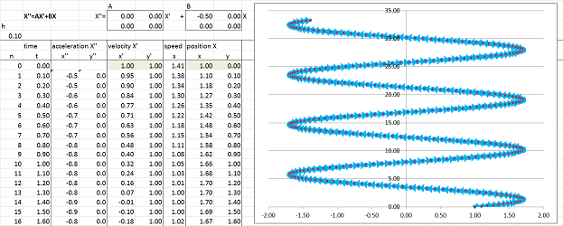
We start with nothing but a spring along the $x$-axis: $$A=\left[\begin{array}{rr} 0&0 \\ 0&0 \end{array}\right], \quad B=\left[\begin{array}{rr} \bf{-0.5}&0\\ 0&0 \end{array}\right].$$

The result is an oscillation along the $x$-axis and uniform motion along the $y$-axis.

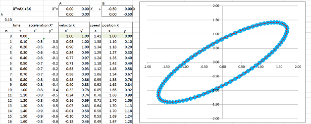
We now add an identical spring for the $y$-axis: $$A=\left[\begin{array}{rr} 0&0 \\ 0&0 \end{array}\right], \quad B=\left[\begin{array}{rr} -0.5&0\\ 0&\bf{-0.5} \end{array}\right].$$

As a result, both $x$ and $y$ oscillate at the same period and come back simultaneously; it's a cycle. The path appears to be an ellipse centered at the origin. We also notice that the motion is slows down at the tips of this ellipse.

Exercise. Why isn't the trajectory a circle?

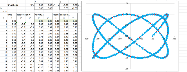
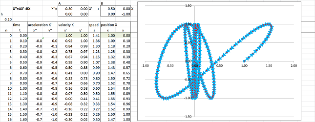
Let's make the latter spring more rigid: $$A=\left[\begin{array}{rr} 0&0 \\ 0&0 \end{array}\right], \quad B=\left[\begin{array}{rr} -0.5&0\\ 0&\bf{-1} \end{array}\right].$$

As a result, $x$ and $y$ still oscillate but at different frequencies. They may come back simultaneously after several periods. That will create a cycle.

We now add friction in the $x$-direction: $$A=\left[\begin{array}{rr} \bf{-0.3}&0\\ 0&0 \end{array}\right], \quad B=\left[\begin{array}{rr} -0.5&0\\ 0&-1. \end{array}\right].$$

While $y$ still oscillates, the $x$-position's oscillation diminishes as it approaches $0$.

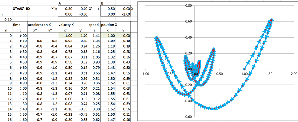
We also add friction in the $y$-direction now: $$A=\left[\begin{array}{rr} -0.3&0\\ 0&\bf{-0.2} \end{array}\right], \quad B=\left[\begin{array}{rr} -0.5&0\\ 0&-1.0 \end{array}\right].$$

Both $x$ or $y$ oscillations diminish and the point approaches $0$.

Up until now, $x$ and $y$ has been independent and the two ODEs are solvable separately. This is why everything we see in the simulations are confirmed by the classification in the last section. From now on, this classification doesn't apply anymore. Note also that the clever trick of introducing the velocities as new variables will produce $4\times 4$ matrices, the analysis of which lies outside the scope of this text. This is why we proceed with discrete models only.

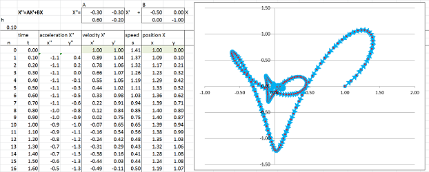
We intermix the two variables now by making the friction vary in the directions other than the two axes (for example, the springs may be placed under various angles): $$A=\left[\begin{array}{rr} -0.3&\bf{-0.3} \\ \bf{0.6}&-0.2 \end{array}\right], \quad B=\left[\begin{array}{rr} -0.5&0\\ 0&-1 \end{array}\right].$$

The pattern of back-and-forth convergence toward $0$ remains.

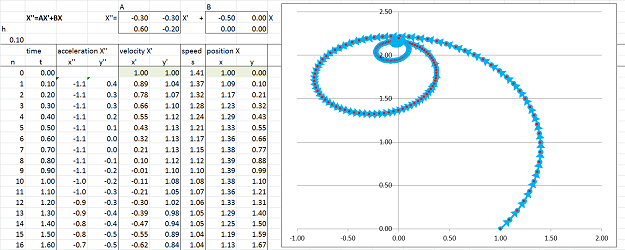
As a final experiment, we remove the $y$-axis spring: $$A=\left[\begin{array}{rr} -0.3&-0.3\\ 0.6&-0.2 \end{array}\right], \quad B=\left[\begin{array}{rr} -0.5&0\\ 0&\bf{0} \end{array}\right].$$

The oscillation of the $y$-coordinate moves away from $0$.

Let's look at what happens to the energy in this discrete model. But first let's see what the data tells about the continuous motion.

For simplicity we continue to assume that the mass is equal to $1$. Then the kinetic energy is known to be this function of time: $$K(t)=\frac{1}{2}||X'(t)||^2.$$ Euler's method samples the velocity and gives us an approximation of this function, the sampled kinetic energy: $$K_n=\frac{1}{2}||X_n'||^2,$$ in each row of the spreadsheet. Next, suppose that the force is conservative. Then the potential energy can be found as the work of this force: $$W(t)=-\int_0^t X' '\cdot X'\, dt.$$ What does the data tell us about this function? Once again, Euler's method samples the velocity and gives us an approximation of this function, the sampled potential energy computed as follows. Over a period of time from $t_{k-1}$ to $t_{k}$ (length $\Delta t$), the potential energy grows by: $$W_k=-X_k' '\cdot X_k'\, \Delta t.$$ We add these in all rows up to the $n$th to find the current sampled potential energy: $$P_n=\sum_{k=0}^n W_k.$$ The next column contains the sum of the two, the total sampled energy: $$E_n=K_n+P_n=\frac{1}{2}||X_n'||^2-\sum_{k=0}^n X_k' '\cdot X_k'\, \Delta t.$$ As you can see, it's not conserved!

The result is to be expected from sampling (a discrete approximation of) a continuous motion.

Definition. A discrete ODE of second order is given by the following recursive formulas: $$\begin{array}{lll} X_{n+1}' '=f(X_n,X_n');\\ X_{n+1}'=X_n'+X_{n+1}' '\, \Delta t;\\ X_{n+1}=X_n+X_{n+1}'\, \Delta t, \end{array}$$ for some function $f$ and a non-zero number $\Delta t$. Its solution is three sequences of vectors that satisfies these equations.

The discrete ODE conserves energy if we just look at the work the right way. We recompute the potential energy in the next column with the current velocity $X_k'$ replaced with the average of the current and the previous velocities: $$W_k=X_k' '\cdot \frac{1}{2}(X_{k-1}'+X_k')\, \Delta t.$$ The last column confirms the conservation of energy. This fact is also easy to prove algebraically for all linear or non-linear discrete systems.

Theorem (conservation of energy). The energy of a solution $X$ of a discrete ODE of second order defined as $$E_n=\frac{1}{2}||X_n'||^2-\sum_{k=0}^n X_k' '\cdot \frac{1}{2}(X_{k-1}'+X_k')\, \Delta t,$$ is constant.

Proof. $$\begin{array}{lll} E_{n+1}-E_n&=\frac{1}{2}||X_{n+1}'||^2-\frac{1}{2}||X_n'||^2-X_{n+1}' '\cdot \frac{1}{2}(X_{n}'+X_{n+1}')\, \Delta t\\ &=\frac{1}{2}\left( ||X_{n+1}'||^2-||X_n'||^2\right)-\frac{1}{\Delta t}\left(X_{n+1}'-X_n'\right)\cdot \frac{1}{2}(X_{n+1}'+X_{n}')\, \Delta t\\ &=\frac{1}{2}\left( ||X_{n+1}'||^2-||X_n'||^2\right)-\frac{1}{2}\left(X_{n+1}'\cdot X_{n+1}' -X_n'\cdot X_n'\right)\\ &=0. \end{array}$$ $\square$

A pendulum

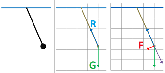
Description: “an object is attached to a fixed point with a string and subjected to the gravity”.

Let $x$ be the horizontal axis and $z$ the vertical.

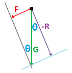
We compute what's necessary, i.e., the acceleration, for the spreadsheet discussed above. Suppose the length of the string is $L$. First, the gravity is the constant vector $$G=<0,-gm>.$$ Then the resistance $R$ of the string is found as the negative of the projection of the gravity on the line from $0$ to the current location $X=<x,z>$: $$R=-\frac{G\cdot X}{||X||^2}X=-\frac{G\cdot X}{L^2}X.$$ Then we find the tangential component of the gravity: $$F=R+G.$$ Or, it is simply: $$F=G\sin \theta,$$ where $\theta$ is the angle of the string with the vertical. Note that the horizontal component of the force is zero when the string is vertical and when it is horizontal and it reverses its direction. Meanwhile, the vertical component is always negative. And the tangential acceleration is: $$A=F/m.$$

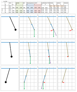
These quantities are computed in that order just as before. The updated values of the velocities and the locations are also found except $z$ is found from $x$ by: $$x^2+y^2=L^2,$$ where $L$ is the length of the string. Equivalently, $$x=L\cos \theta,\ y=L\sin\theta.$$ We use a spreadsheet to evaluate these column by column and then for each iteration of $t$:

The visualization suggests that we indeed have a pendulum.

For the $3$-dimensional case, we give the pendulum another -- horizontal -- degree of freedom, $y$. The vector analysis remains the same with $G=<0,0,-gm>$ and $X=<x,y,z>$. The spreadsheet only requires adding columns for $y$. The values of $z$ is found from: $$x^2+y^2+z^2=L^2.$$ Below we plot the parametric curve $<x,y>$ with a non-zero horizontal component of the initial velocity:

We observe that the pendulum swings as before but the plane of the swings is continuously rotating.

We now go back to the $2$-dimensional case and address it analytically. We apply Newton's law to the tangential axis only: $$F = -mg\sin\theta = ma\ \Longrightarrow\ a= -g \sin\theta.$$ How is this linear acceleration $a$ along the tangent related to the change in angle $\theta$? Let $s$ be the arc-length parameter. Since the curve is a circle of radius $L$, we have: $$s = L\theta.$$ Now, the arc-length parameter is a function of $t$, i.e., $s=s(t)$. We differentiate twice with respect to $t$: $$s = L\theta\ \Longrightarrow\ v=s' = L\theta'\ \Longrightarrow\ a = x' ' = L\theta' '.$$ Therefore, $$L\theta' ' = -g \sin\theta,$$ or $$\theta' ' + \frac{g}{L} \sin\theta = 0. $$ This is a non-linear ODE with respect to $\theta$.

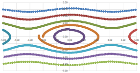
To confirm our simulations, we plot a few solutions using Euler's method just as in the last chapter:

Here $\theta$ is plotted against $\alpha=\theta'$; i.e., we are considering the following system: $$\begin{cases} \theta'=\alpha,\\ \alpha'=-\frac{g}{L} \sin\theta. \end{cases}$$ The Euler's solutions aren't periodic but rather appear to be spirals!

Let's linearize! There is only one equilibrium $\theta =\alpha =0$. Now, $$\frac{d}{d\theta}\big( \sin\theta \big)(0)=1.$$ Therefore, the linearized systems is: $$\begin{cases} \theta'=\alpha,\\ \alpha'=-\frac{g}{L}\theta. \end{cases}$$ We can look at the eigenvalues: $$A=\left[\begin{array}{ll} 0&1\\ -\frac{g}{L}&0 \end{array}\right] \ \Longrightarrow\ \chi_A(\lambda)=\det(A-\lambda I)=\det\left[\begin{array}{ll} -\lambda&1\\ -\frac{g}{L}&-\lambda \end{array}\right]=\lambda^2+\frac{g}{L}=0 \ \Longrightarrow\ \lambda_{1,2}=\pm\sqrt{\frac{g}{L}}i.$$ According to the Classification of linear systems II in Chapter 23, the system has a center at $0$! Of course, we can just solve the linearized system: $$\theta' '=\alpha'=-\frac{g}{L}\theta\ \Longrightarrow\ \theta=\theta_0\cos\left( \sqrt{\frac{g}{L}}t \right),$$ with the initial conditions: $$\theta(0)=\theta_0 \text{ and } \theta'(0)=0.$$ So, our conclusion is that when small the swings are close to periodic with a period $2\pi\sqrt{\frac{g}{L}}$. The period is independent of the amplitude $\theta_0$!

Planetary motion

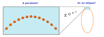
A familiar problem about a ball thrown in the air has a solution: its trajectory is a parabola. However, we also know that if we throw really-really hard (like a rocket) the ball will start to orbit the Earth following an ellipse.

The motion of two planets (or a star and a planet, or a planet and a satellite, etc.) is governed by a single force: the gravity. Recall how this force operates.

Newton's Law of Gravity: The force of gravity between two objects is

• 1. proportional to either of their masses,
• 2. inversely proportional to the square of the distance between their centers, and
• 3. directed along the segment between them.

In other words, the force is given by the formula: $$F = G \frac{mM}{r^2},$$ where:

• $F$ is the force between the objects;
• $G$ is the gravitational constant;
• $m$ is the mass of the first object;
• $M$ is the mass of the second object;
• $r$ is the distance between the centers of the masses.

Let's connect this familiar physics law to another.

Kepler's Laws of Planetary Motion: The motion of planets around the Sun follows these laws:

• 1. The orbit of a planet is an ellipse with the Sun at one of the two foci.
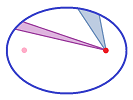
• 2. A line segment joining a planet and the Sun sweeps out equal areas during equal intervals of time.
• 3. The square of the orbital period of a planet is proportional to the cube of the semi-major axis of its orbit.

We know the vector form of Newton's law (with the first object located at the origin): $$F=-G mM\frac{X}{||X||^3}.$$ Then, we have a vector ODEs of second order for the location $X$ of the second object: $$X' '=-G M\frac{X}{||X||^3}.$$ We will call it Newton's ODE of planetary motion. It is non-linear.

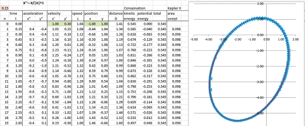
As before, from the acceleration $X' '_n$ the velocity $X'_n$ and then from the velocity the position $X_n$ are computed by what amounts to Euler's method. The discrete model of planetary motion is a discrete model of second order given by the following recursive formulas: $$\begin{array}{lll} X_{n+1}' '=-G M\frac{X_n}{||X_n||^3};\\ X_{n+1}'=X_n'+X_{n+1}' '\, \Delta t;\\ X_{n+1}=X_n+X_{n+1}'\, \Delta t. \end{array}$$ The result is as predicted: the points form what looks like an ellipse with one of the foci at the origin (First Kepler's Law).

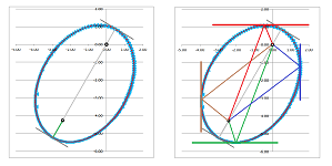
In order to confirm this idea, we first draw a line from the origin (the first focus) to the point on the curve where it is perpendicular to the tangent. We then continue this line to the other end of the curve and discover that indeed the tangent is again perpendicular to this chord. We then measure the distance from the focus to the first point and plot the same distance from the second point along the chord. This gives us the second focus (left).

We further test our conjecture by plotting the lines representing rays of light that start at one focus and then bounce off the curve to the other focus (right).

Exercise. Is this really an ellipse?

By changing the initial conditions we can produce other patterns of behavior such as what looks like a hyperbola:

Now what about the Second Kepler's Law?

We can see in our simulation that the points away from the origin (the first object) are closer spaced than the ones closer to the origin. This means that the motion is faster when they are closer. That is why the longer triangles are thinner.

We confirm that the areas of the triangles are the same by computing them in the last column of the spreadsheet via the Parallelogram Formula: $$A_{n+1}=\frac{1}{2}\big|\det \left[ X_{n+1}X_n \right]\big|,$$ where $X_{n+1}$ and $X_n$ are given by their column vectors.

We will derive the law in a more general setting than the original. First we note that it might apply to all discrete trajectories not just ellipses.

Exercise. Prove that an object moving along a straight line at a constant speed satisfies the area property with respect to any fixed point. Hint: use elementary geometry.

Second, we will see that the law applies to more general forces than just the gravity. The gravity is a central force, i.e., one that is directed along the line between the location and the origin. Then the recursive formula for such a discrete models is: $$X_{n+1}' '=L(||X_n||)X_n,$$ for some function $L$.

Theorem (Discrete Second Kepler's Law). If $X$ is a trajectory of the discrete model with central force, the segment from the focus to the location sweeps an equal area in an equal time. Conversely, if this area property is satisfied by each trajectory of a discrete model of order two, the model is produced by a central force.

Proof. We consider the model: $$X_{n+1}' '=f(X_n),$$ where $f$ is some function. Then, $$X_{n+1}'=X_n'+X_n' ' \Delta t=X_n'+f(X_n)\Delta t.$$

We will use twice the Parallelogram Formula for the oriented area $A$ of the triangle spanned by vectors $M$ and $N$: $$A=\frac{1}{2}\det \left[ M\,N \right].$$ However, the vectors chosen will be different from those used in the spreadsheet.

First, suppose the triangle with area $A_{n}$ is formed by $X_n$ and $X_{n}'\Delta t$; therefore, we have by the linearity of the determinant: $$A_{n}=\frac{\Delta t}{2}\det \left[X_n\,X_{n}'\right] .$$

Second, suppose the triangle with area $A_{n+1}$ is formed by $X_n$ and $X_{n+1}'\Delta t$; therefore, we have the following by the linearity and the additivity of the determinant: $$\begin{array}{ll} A_{n+1}&=\frac{\Delta t}{2}\det \left[X_n\ X_{n+1}'\right] \\ &=\frac{\Delta t}{2}\det \left[X_n\ (X_n'+f(X_n)\Delta t) \right] \\ &=\frac{\Delta t}{2}\big( \det \left[X_n\ X_n'\right]+\Delta t\det \left[X_n\ f(X_n)\right]\big) .\\ \end{array}$$

Therefore, $$A_{n+1}-A_n=\frac{\Delta t^2}{2}\det \left[X_n\ f(X_n)\right].$$ Finally, $A_{n+1}=A_n$ if and only if $X_n$ and $f(X_n)$ are parallel. $\blacksquare$

Exercise. Derive Kepler's Second Law from this theorem. Hint: use what you know about the accuracy of Euler's method.

We thus conclude that the motion along the ellipse (or the parabola, or the hyperbola seen below) does not match its standard parametrization, $x=a\sin \omega t,\ y=b\sin \omega t$.

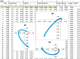
The formulas fully apply to the $3$-dimensional situation. Plotting the orbit along the three coordinate planes produces the following:

Exercise. Implement a simulation of planetary motion in the $3$-dimensional space. Demonstrate that the motion is planar.

We state the following without proof.

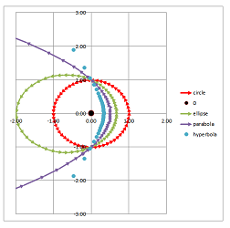
Theorem. Any trajectory of the Newton's ODE of planetary motion is given by the following in polar coordinates: $$r=\frac{p}{1+e \cdot\cos \theta},$$ which is

• a circle for $e=1$,
• an ellipse for $0 <e <1$,
• a parabola for $e = 1$,
• a hyperbola for $e > 1$,

with the focus at the origin.

The graphs are plotted for $e = 0,.5,1,2$:

The proof of this theorem lies beyond the scope of this book.

Finally, let's go back to the question posed in the beginning of the section: what is the correct trajectory?

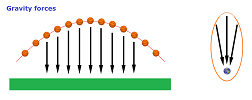
Let's review what we concluded about these two settings in Chapter 17.

• When the Earth is seen as “large” in comparison to the size of the trajectory, the gravity forces are assumed to be parallel in all locations. Then the trajectory is a parabola as the graph of a function with the $x$-axis aligned with the surface of the Earth and $y$-axis with the force.
• When the Earth is seen as either “small” or at least perfectly spherical, the gravity forces are assumed to go radially toward its center. Then the trajectory is an ellipse (or a hyperbola or a parabola) with its focus located at the center.

When the size and, therefore, the shape of the Earth matter, things get complicated...

The two- and three-body problems

We have ignored the effect of the Earth's gravity on the Sun. The reason is that the mass $p$ of the Sun is significantly larger than the mass $q$ of the Earth: $$p>>q.$$ This is the assumption that allows us to place the Sun at the origin as a stationary object. What if we have the two planets of comparable sizes?

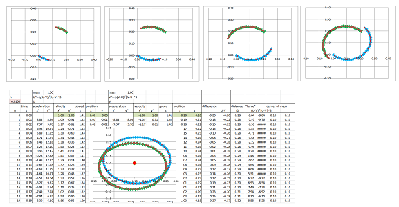
Suppose now we have two planets with masses $p,q$ with located at $U,V$ respectively. Either of the two objects is affected by the gravity of the other. Then the two interactions appear in the two dependent ODEs: $$\begin{array}{lll} U' '=-G q\frac{U-V}{||U-V||^3};\\ V' '=-G p\frac{V-U}{||V-U||^3}.\\ \end{array}$$ This is called the two-body problem.

Let's apply Euler's method to see what can happen.

We start with two identical planets. They seem to circle each other...

...until we realize that either one circles a certain point, the same point for both. This point lies half-way between then, $$C=\frac{1}{2}(U+V).$$ This fact is confirmed in the last column of the spreadsheet.

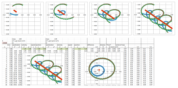
Let's double the mass of the first planet. With everything else remaining the same, the two planets seem to dance away while still circling each other. This time, the mid-point is also circling.

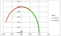
In fact, it doesn't seem to reveal anything about what is going on. What if we look at the center of mass of the two, $$M=\frac{p}{p+q}U+\frac{q}{p+q}V,$$ instead? It seems to be moving along a straight line!

Furthermore, let's plot the two trajectories with respect to the center of mass, i.e., $$P=U-M \text{ and } Q=V-M.$$ They seem to trace ellipses.

Let's state and prove these conjectures.

Theorem. The center of mass $M$ of the two-body system satisfies the vector ODE: $$M' '=0,$$ and, therefore, moves along a straight line at a constant speed.

Proof. We simply substitute: $$\begin{array}{ll} M' '&=\left( \frac{p}{p+q}U+\frac{q}{p+q}V \right)' '\\ &= \frac{p}{p+q}U' '+\frac{q}{p+q}V ' '\\ &= \frac{p}{p+q}\left(-G q\frac{U-V}{||U-V||^3}\right)+\frac{q}{p+q}\left(-G p\frac{V-U}{||V-U||^3}\right)\\ &=-G\frac{pq}{p+q}\left(\frac{U-V}{||U-V||^3}+\frac{V-U}{||U-V||^3}\right)\\ &=0. \end{array}$$ $\blacksquare$

Theorem. If $U$ and $V$ are the locations of the two planets in the two-body system and $M$ is its center of mass $M$, then $P=U-M$ and $Q=V-M$ satisfy the Newton's ODE of planetary motion and, therefore, trace ellipses, parabolas, or hyperbolas.

Proof. We first observe that $M$ located on the line between $U$ and $V$ in proportion to their masses. Therefore, $U-V$ is proportional to $U-M$: $$M=\frac{p}{p+q}U+\frac{q}{p+q}V\ \Longrightarrow\ U-V=\frac{p+q}{q}(U-M).$$ Now, we simply substitute: $$\begin{array}{ll} P' '&=(U-M)' '\\ &=U' ' - M' '\\ &=-G q\frac{U-V}{||U-V||^3} - 0\\ &=-G q\frac{\frac{p+q}{q}(U-M)}{||\frac{p+q}{q}(U-M)||^3} \\ &=-G q\frac{U-M}{\left(\frac{p+q}{q}\right)^2||(U-M)||^3} \\ &=-G q\left(\frac{q}{p+q}\right)^2 \frac{U-M}{||(U-M)||^3} \\ &=-G \frac{q^3}{(p+q)^2} \frac{P}{||P||^3} . \end{array}$$ $\blacksquare$

In the last example, we go back to the case of two identical planets and simply increase the $y$-component of the velocity of the second planet from $1$ to $2$. With a certain amount of circling, they start to move away from each other.

Eventually, they are flying in the opposite directions! Just as in the last case, plotting the trajectories with respect to the center of mass help to reveal the pattern.

Thus, depending on the initial conditions, these three seem to be the most interesting outcomes. In the first, two identical planets dance around each other (in reality, around the combined center of mass). In the second, they dance away together (still around the center of mass, which is moving). Finally, the two run away from each other because beyond some distance they feel almost no pull...

Exercise. Why don't any of the planets in the solar system behave this way? What other possibilities can you think of?

What about three planets?

First let's review a related problem discussed in Chapter 17. The fact that the Earth orbits the Sun and the Moon orbits around the Earth may be illustrated with the picture on left while the actual data about the dimensions of the orbits and the period of the Moon produce the picture on right:

Suppose now that the three planets have masses $p,q,m$. If we assume that $$p>>q>>m,$$ such as in the case of Sun-Earth-Moon, the effect of the gravity of the second on the first and the third on the second is negligible, just as in the last section. Suppose

• $U=0$ is the location of the Sun fixed at the origin,
• $V$ is the location of the Earth with respect to the Sun, and
• $X$ is the location of the Moon with respect to the Earth.

Then the two interactions are independent of each other and we have two independent Newton's ODEs of planetary motion: $$\begin{array}{lll} V' '=-G p\frac{V}{||V||^3};\\ X' '=-G q\frac{X}{||X||^3}. \end{array}$$ Both solutions follow their respective ellipses. We then add them as vectors, $$W=V+X,$$ to produce the path of the third planet around the first. Generically, it looks like this:

We next make one generalization: the mass of the second planet is not negligibly small relative to that of the first anymore. We, then, can't fix the first at the origin anymore. We have a two-body system just as above: $$\begin{array}{lll} U' '=-Gq\frac{U-V}{||U-V||^3};\\ V' '=-Gp\frac{V-U}{||V-U||^3};\\ W' '=-Gp\frac{W-U}{||W-U||^3}-q\frac{W-V}{||W-V||^3}. \end{array}$$ In the meantime, the third planet is affected by the gravity of the first two. It is called the restricted three body problem

While the two first planets do the same, the variety of behaviors of the third is enormous even in dimension $2$:

There are many periodic trajectories but we will point out only one. Below we confirm that it is possible to place a satellite on the Moon's orbit, $60$ degrees ahead, that will continue to revolve in this fashion indefinitely.

Now, in general. Suppose now we have three planets with masses $m_1,m_2,m_3$ located at $V_1,V_2,V_3$ respectively. Each of the three objects is affected by the gravity of either of the other two. Then these three interaction appear in the three dependent vector ODEs: $$\begin{array}{lll} V_1' '=-G m_2\frac{V_1-V_2}{||V_1-V_2||^3}-G m_3\frac{V_1-V_3}{||V_1-V_3||^3};\\ V_2' '=-G m_1\frac{V_2-V_1}{||V_2-V_1||^3}-G m_3\frac{V_2-V_3}{||V_2-V_3||^3};\\ V_3' '=-G m_1\frac{V_3-V_1}{||V_3-V_1||^3}-G m_2\frac{V_3-V_2}{||V_3-V_2||^3}. \end{array}$$ The general three body problem has no analytic solution.

A cannon is fired...

What we know about history of ballistics is that the parabolic trajectories were known since Galileo and, furthermore, Newton worked out the physics behind and the mathematics (calculus) behind this idea. Nonetheless, as recently as mid-19th century they aimed cannons based entirely on the information that comes from experimentation, without mathematics.

Here is an excerpt from The Emperor Napoleon's New System of Field Artillery (1854):

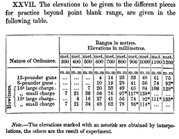
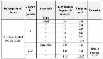
Below is the “range table” from the The Confederate Ordnance Manual during the American Civil War (1860s). Clearly, the numbers come from shooting and then measuring the distance:

With what we know about the dynamics of projectiles, we can try to reproduce these results.

We start with the same initial value problem: $$\begin{cases} x' '&=0\\ y' '&=-32 \end{cases},\quad \begin{cases} x'(0)&=s_0\cos\alpha\\ y'(0)&=s_0\sin\alpha \end{cases},\quad \begin{cases} x(0)&=0\\ y(0)&=y_0 \end{cases},$$ where $s_0$ is the initial speed and $\alpha$ is the angle of the barrel.

Example. The initial value problem has already been solved: $$\begin{cases} x&=&\quad s_0\cos\alpha\cdot t,\\ y&=y_0&+s_0\sin\alpha\cdot t&-16t^2. \end{cases}$$ We need to find such an $x$ that $y=0$. We find the time to reach the ground first (choosing the positive value): $$t=\frac{-s_0\sin\alpha\pm\sqrt{(s_0\sin\alpha)^2-4(-16)y_0}}{2(-16)}=\frac{1}{32}\left(s_0\sin\alpha+\sqrt{(s_0\sin\alpha)^2+64y_0}\right).$$

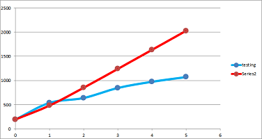
We consider the 12-pound field howitzer. Suppose the muzzle velocity is known, $s_0=1054$ feet per second. We also estimate the initial elevation (the height of the cannon) at $y_0=5$ feet. Then the distances should be: $$\begin{array}{c|ccc|c} \text{elevation in degrees}&\text{time in seconds, }t&\text{distance in feet, }x&\text{distance in yards}&\text{test distance}\\ \hline 0&0.56 &589 &196 &195\\ 1&1.38 &1451 &484 &539\\ 2&2.43 &2557 &852 &640\\ 3&3.54 &3722 &1241 &847\\ 4&4.66 &4902 &1634 &975\\ 5&5.80 &6085 &2028 &1072 \end{array}$$ We see a mismatch with the data that grows fast with the angle.

$\square$

Exercise. Explain why the red curve looks straight.

The reason why the Newtonian mechanics overestimates the distance is known; it is the air-resistance. In fact, Newton himself worked out all necessary details of ballistics including taking into account the air resistance. He assumed however that the resistance force is proportional to the speed. Half a century later Euler thought, for ballistics, it is better to take the resistance force is proportional to the square of the speed. That was 100 years before those tests!

The drag equation gives the force $F_D$ of drag experienced by an object due to its movement through the air: $$||F_D|| = \tfrac12 \rho CA \cdot s^2,$$ where

• $\rho$ is the density of the air,
• $A$ is the cross sectional area of the projectile,
• $C$ is the drag coefficient – a dimensionless coefficient that depends on the projectile's geometry, and
• $s$ is the speed of the projectile.

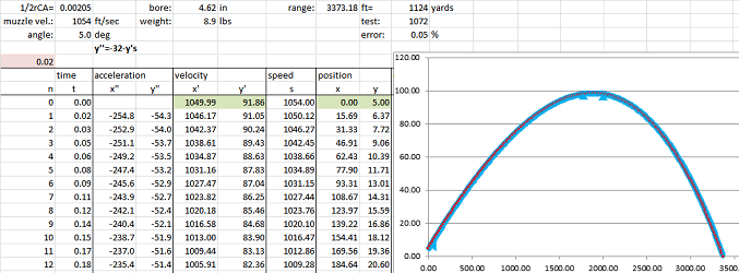
The direction of this force $F_D$ and, therefore, that of the acceleration is opposite to the direction of the velocity $X'$. Therefore, the acceleration generated by this force is $$-\tfrac12 \rho CA\frac{1}{M} sX',$$ where $M$ is the mass of the projectile. Then our IVP becomes: $$\begin{cases} x' '&=&-\tfrac12 \rho CA\frac{1}{M} sx'\\ y' '&=-32&-\tfrac12 \rho CA\frac{1}{M} sy' \end{cases},\quad \begin{cases} x'(0)&=s_0\cos\alpha\\ y'(0)&=s_0\sin\alpha \end{cases},\quad \begin{cases} x(0)&=0\\ y(0)&=y_0 \end{cases}.$$ With this updated dynamics of projectiles, let's try again to reproduce the test results.

Example. We need some information for the drag equation:

• the weight $M=8.9$ pounds,
• the area $A=\pi r^2$ of the cross section of the cannonball, where the radius is $r=4.62/2=2.31$ inches,
• the density of the air $\rho = 0.074887$ pounds per cubic foot,
• the drag coefficient of a sphere $C=.47$.

We use Euler's method:

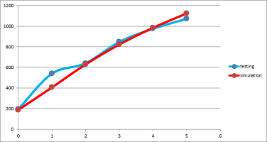
We repeat it for each elevation, six times: $$\begin{array}{c|c|c} \text{elevation in degrees}&\text{distance in yards}&\text{test distance}\\ \hline 0 &187 &195\\ 1 &405 &539\\ 2 &629 &640\\ 3 &822 &847\\ 4 &984 &975\\ 5 &1124 &1072 \end{array}$$ Much better!

$\square$

Boundary value problems

Example. Setting differential equations aside for a moment, let's consider this simple problem:

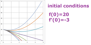
• from all quadratic polynomials $f(x)=ax^2+bx+c$, find ones with $f(0)=20,\ f'(0)=-3$.

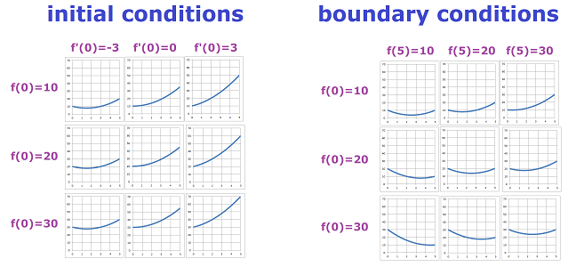
Here, the value of the function and its derivative are provided for a particular value of the variable, $x=0$. These are called initial conditions. The word “initial” refers to the starting point, $0$, of the ray $[0,\infty]$.

Let's change the problem:

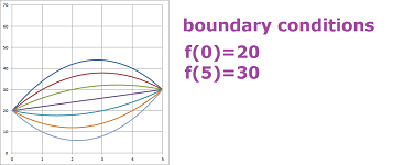
• from all quadratic polynomials $f(x)=ax^2+bx+c$, find ones with $f(0)=20,\ f(5)=30$.

In this case, the value of the function is provided for two values of $x$ and no values of the derivative are provided. These are called boundary conditions. The word “boundary” refers to the end-points, $0$ and $5$, also known as the boundary points, of the interval $[0,5]$.

$\square$

Exercise. Find all these polynomials.

Example. Let's limit ourselves to quadratic polynomials with $a=1$:

• from all quadratic polynomials $f(x)=x^2+bx+c$, find the one with $f(0)=20,\ f'(0)=-3$; and
• from all quadratic polynomials $f(x)=x^2+bx+c$, find the one with $f(0)=20,\ f(5)=30$.

Then we have a certain uniqueness, i.e., there is only one answer to the question; the solution in the former case is, of course, $c=20,\ b=-3$. For the latter case we need more algebra: $$c=20\ \Longrightarrow\ 5^2+ b\cdot 5+20=30\ \Longrightarrow\ b=(30-5^2-20)/5=3.$$

$\square$

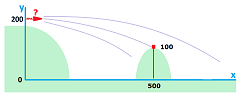
Example. Let's review a familiar problem from Chapters 1 and 7. From a $200$ feet elevation, a cannon is fired horizontally at $200$ feet per second. How far will the cannonball go?

We know this as an initial value problem. Indeed, the ODE has been solved: $$\begin{cases} x&=&200t,\\ y&=200&&-16t^2. \end{cases}$$ Now we just need to find the solution that satisfies the initial conditions:

• the initial location: $X(0)=(x(0),y(0))=(0,200)$;
• the initial velocity: $X'(0)=(x'(0),y'(0))=(200,0)$.

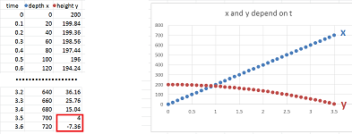
We scroll down the spreadsheet to find the row with $y$ close to $0$: around $t_1=3.55$ seconds, with the value of $x$ at the time close to $710$ feet. Algebraically, we solve an equation and then substitute: $$y(t_1)=200-16t_1^2=0\ \Longrightarrow\ t_1=\sqrt{\frac{200}{16}}=\frac{5\sqrt{2}}{2}\ \Longrightarrow\ x_1=x(t_1)=200t_1=200\frac{5\sqrt{2}}{2}\approx 707.$$

Now what could be the meaning of boundary conditions in this setting? We already have one, the initial location. The second may be the final location when, for example, we are trying to hit a target -- at a particular moment of time. Suppose we want the cannon ball to be at $(200,500)$ after $2$ seconds. In that case the muzzle velocity of the cannon is unspecified and it is what we are supposed to find. We thus need to find a solution (there could be one, many, or none) that satisfies the boundary conditions:

• the first boundary location: $X(0)=(x(0),y(0))=(0,200)$;
• the second boundary location: $X(2)=(x(2),y(2))=(500,100)$.

This is called a boundary value problem. Let's solve it.

Where do the solutions come from? The ODE has been solved and the first boundary condition gives us the initial location: $$\begin{cases} x&=x_0&+ut&\\ y&=y_0&+vt&-16t^2 \end{cases} \ \Longrightarrow\ \begin{cases} x&=0&+ut&\\ y&=200&+vt&-16t^2 \end{cases}.$$ We now find $u,v$ from the second boundary condition. One dimension at a time: for $x$, $$x(2)=v \cdot 2=500\ \Longrightarrow\ u=250;$$ and for $y$, $$y(2)=200+v\cdot 2-16\cdot 2^2=100\ \Longrightarrow\ 2v=100-(200-16\cdot 2^2)\ \Longrightarrow\ v=(-100+16\cdot 4)/2=-18.$$ Note that a more practical situation is when the muzzle velocity, mathematically the speed, remains the same and it is the angle of the barrel that we need to find. $\square$

Example. Consider the familiar ODE for the oscillation of an object on a spring: $$y' '(x)+y(x)=0.$$ But this time we aren't trying to predict what happens to the object with known position and velocity. We ask ourselves if the system can bring the object from a particular position to another in a specific amount of time, for example: $$y(0)=0, \ y(\pi/2)=2.$$ The general solution to our ODE is $$y(x) = A \sin x + B \cos x.$$ Now, from the first boundary condition we obtain: $$0 = A \cdot 0 + B \cdot 1\ \Longrightarrow\ B=0.$$ From the boundary condition we obtain: $$2 = A \cdot 1 \ \Longrightarrow\ A=2.$$ Thus imposing these boundary conditions produces a unique solution: $$y(x)=2\sin x. $$ $\square$

When the functions have two or more variables, regions are more complicated and so are their boundaries. Such differential equations are beyond the scope of this book.

Reflecting light

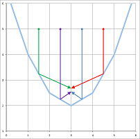
In the beginning of Chapter 5, we used fact that the light bouncing from a parabolic mirror will all meet at one point as an example of how the Tangent Problem may emerge. We traced how the light bounces off the secant lines of a parabola:

First, suppose there is only a straight surface. We let the light drop vertically on a straight line, where does it go from there?

File:Vertical light bounces off.png

Theorem. The angle between a vertical vector $<0,1>$ and vector $<1,m>$ (slope $m$) and the angle between $<0,1>$ and a unit vector $<a,b>$ is the same when $$a=\frac{2m}{m^2+1},\ b=\frac{m^2-1}{m^2+1}.$$

Proof. The dot product should be the same: $$<1,m><a,b>=<1,m><0,1>,$$ or $$a+mb=m\ \Longrightarrow\ a=m(1-b).$$ Since this is a unit vector, we have: $$a=\sqrt{1-b^2}=m(1-b)\ \Longrightarrow\ 1-b^2=m^2(1-b)^2\ \Longrightarrow\ (1-b)(1+b)=m^2(1-b)^2.$$ We cancel $1-b$ now because $b=1$ would give us the original vertical vector. Then, $$1+b=m^2(1-b)=m^2-m^2b\ \Longrightarrow\ b=\frac{m^2-1}{m^2+1}.$$ $\blacksquare$

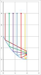
Following the theorem, we test the property of the parabola by bouncing off the light off some of its secant lines:

The pattern is clear but this is just an approximation!

Exercise. When is the angle between a vector $<p,q>$ and vector $<n,m>$ and the angle between $<p,q>$ and a unit vector $<a,b>$ the same?

We now approach this construction from the opposite direction:

• what curves have this property?

Suppose the point $F$ of convergence of light is given. Suppose we also have a point $A=(x_0,y_0)$ where an edge of the mirror is to start. Now, what is the slope $m$ of the line starting at $A$ that will bounce a vertical ray $y=x_0+h$ light to $F$?

A source of light placed at the focus of a parabola will create a beam of parallel rays of light (headlights).