Treat calculus discretely!

Redirect to:

• Sequences and their limits

What is calculus about?

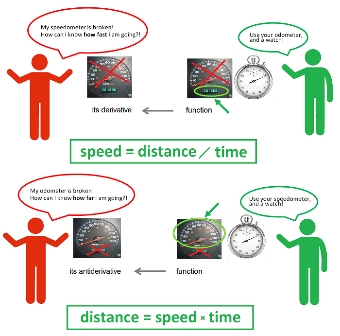
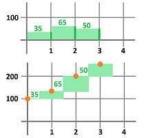
This is what happens in an elementary calculus shown in a single picture:

Let's consider two specific situations.

Suppose the speedometer is broken. If now we want to estimate how fast we are driving, we look at the odometer at several moments and record the mileage. For example, if we look every hour, we may have this:

• initial reading: $10,000$ miles;
• after the first hour: $10,055$ miles;
• after the second hour: $10,095$ miles;
• after the third hour: $10,155$ miles;
• etc.

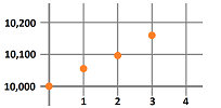
Let's plot our location as a function of time:

As we see, the unknown location function has been sampled.

Now, the speed. We rely on the well-known formula $$\text{ speed }= \frac{\text{ distance }}{\text{ time }}.$$ The time period was chosen to be $1$ hour, so we need only to look at the distance covered during each of these one-hour periods:

• distance during the first hour: $10,055-10,000=55$ miles;
• distance during the second hour: $10,095-10,055=40$ miles;
• distance during the third hour: $10,155-10,095 =60$ miles;
• etc.

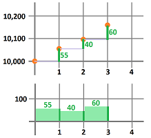
These three numbers give us the average speed of our driving for each of the time periods. This is how these new numbers appear in the plot:

As you can see, we treat the outcome data as if the speed remains constant during these hour-long periods.

Now in reverse...

Suppose the odometer is broken. If now we want to estimate how far we have gone, we look at the speedometer at several moments and record its readings. For example, if we look every hour, we may have this:

• during the first hour: $35$ miles an hour;
• during the first hour: $65$ miles an hour;
• during the first hour: $50$ miles an hour;
• etc.

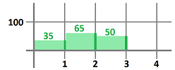
Let's plot our speed as a function of time:

Here, the unknown speed function has been sampled but we treat the data as if the speed remains constant during these hour-long periods.

Now, the location. We use the same formula: $$\text{ distance }=\text{ speed }\times \text{ time }.$$ Suppose also that our trip started at the $100$ mile mark. The time period was chosen to be $1$ hour, so we need only to look at the speed at which -- we assume -- we drove during each of these one-hour periods:

• the location after the first hour: $100+35=135$ mile mark;
• the location after the two hours: $135+65=200$ mile mark;
• the location after the three hours: $200+50=250$ mile mark;
• etc.

This is how these new numbers appear in the plot:

We next consider more detailed examples. Here our ability to use negative numbers allows us to treat the data the same way even when we are moving in the opposite direction. In this case, we are dealing with the velocity instead of the speed.

From location to velocity

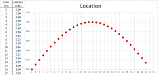
This time we consider about $30$ data points. They are our locations recorded every minute: $$\begin{array}{l|l|llllllllll} \text{ location } & \text{ miles } & 0.00 &0.10 &0.20 &0.30 &0.39 &0.48 &0.56 &0.64 &0.72 &0.78 &0.84 &...\\ \hline \text{ time } & \text{ min } &0 &1 &2 &3 &4 &5 &6 &7 &8 &9 &10 &... \end{array}$$ This data is seen in the first two columns of the spreadsheet:

The data is furthermore illustrated as a scatter plot on the right.

To understand how fast we move over these one-minute intervals, we compute the differences of locations. $$\begin{array}{l|l|llllllllll} \text{ velocity } & \text{ miles/min } &- &0.10 &0.10 &0.10 &0.09 &0.09 &0.09 &0.08 &0.07 &0.07 &0.06 &...\\ \text{ location } & \text{ miles } &0.00 &0.10 &0.20 &0.30 &0.39 &0.48 &0.56 &0.64 &0.72 &0.78 &0.84 &...\\ \hline \text{ time } & \text{ min } &0 &1 &2 &3 &4 &5 &6 &7 &8 &9 &10 &... \end{array}$$

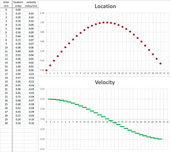
The spreadsheet formula is simple: $$\texttt{ =RC[-1]-R[-1]C[-1]}$$ It is used for each time interval and the data is shown in the next column:

The data is also illustrated as the second scatter plot on the right. To emphasize the fact that the velocity data is referring to time intervals rather than time instances, as the location, we plot it with horizontal segments. In fact, the data table can be rearranged as follows to make this clear: $$\begin{array}{l|c|c|c|c|c|c|c|c|c|c} \text{ velocity } &\cdot&0.10& \cdot&0.10& \cdot&0.10& \cdot&0.09& \cdot&0.09 &...\\ \text{ location } &0.00 &-&0.10 &-&0.20 &-&0.30 &-& .39&-&...\\ \hline \text{ time } &0 &&1 &&2 &&3 &&4 &&... \end{array}$$

What has happened can now be easily read from the second graph:

• the velocity was positive initially and we were moving in the positive direction;
• we were moving fairly fast but then we started to slow down;
• we stopped for a very short period;
• then the velocity became negative as we started to move in the opposite direction;
• we started to speed up in that direction.

Thus the second function succinctly records some facts about the qualitative and quantitative behavior of the former. As the latter is derived from the former, the transition is described by: $$\text{function} \quad \longrightarrow \quad \text{its derivative}$$

From velocity to location

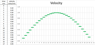
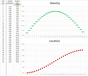
Again, we consider about $30$ data points. They are our velocities recorded every minute: $$\begin{array}{l|l|llllllllll} \text{ velocity }&\text{ miles }&0.00 &0.10 &0.20 &0.30 &0.39 &0.48 &0.56 &0.64 &0.72 &0.78 &0.84 &...\\ \hline \text{ time } &\text{ min } &0 &1 &2 &3 &4 &5 &6 &7 &8 &9 &10 &... \end{array}$$ This data is seen in the first two columns of the spreadsheet:

The data is furthermore illustrated as a scatter plot on the right. Again we emphasize the fact that the velocity data is referring to time intervals and plot it with horizontal bars.

To find out where we are at the end of each of these one-minute intervals, we compute the sums of the velocities. $$\begin{array}{l|l|llllllllll} \text{ location } &\text{ miles/min } &0.00 &0.10 &0.30 &0.59 &0.98 &1.46 &2.03 &2.67 &3.39 &4.17 &...\\ \text{ velocity } &\text{ miles } &-&0.00 &0.10 &0.20 &0.30 &0.39 &0.48 &0.56 &0.64 &0.72 &...\\ \hline \text{ time } &\text{ min } &0 &1 &2 &3 &4 &5 &6 &7 &8 &9 &... \end{array}$$

The spreadsheet formula is simple: $$\texttt{ =R[-1]C+RC[-1]}$$ It is used for each time interval and the data is shown in the next column:

The data is also illustrated as the second scatter plot on the right.

We again rearrange the data table to make the difference between two types of data clear: $$\begin{array}{l|c|c|c|c|c|c|c|c|c|c} \text{ location } &0.00 &-&0.10 &-&0.30 &-&0.59&-& .98&-&...\\ \text{ velocity } &\cdot&0.00& \cdot&0.10& \cdot&0.20& \cdot&0.30& \cdot&0.39 &...\\ \hline \text{ time } &0 &&1 &&2 &&3 &&4 &&... \end{array}$$

Thus, as the former function records some facts about the quantitative behavior of the latter, we are able to combine this information to recover the latter. This backward transition is described by: $$\text{function} \quad \longrightarrow \quad \text{its antiderivative.}$$

The terminology is justified by the fact that the two operations we have considered undo the effect of each other: $$\text{location} \quad \longrightarrow \quad \text{velocity} \quad \longrightarrow \quad \text{same location (up to initial position),} $$ and $$\text{velocity} \quad \longrightarrow \quad \text{location (up to initial position)} \quad \longrightarrow \quad \text{same velocity.} $$

Furthermore, we now use what we understand about the behavior of these discrete functions to describe functions that are seen only as -- possible continuous -- graphs. We simply look at the slope of the graph:

Here we even replace our main metaphor, location, for another, temperature. The results are just as applicable to any other quantity that depends on time, or any other quantity.