The derivative

The Tangent Problem

There are two main ways to enter calculus: through the study of geometry and through the study of motion. In this and next sections, we will discuss the two approaches respectively.

In what direction will light bounce off a curved mirror?

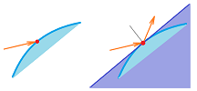
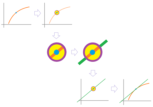
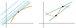
Since the ray is so thin, there is just a single point of contact. Then the light bounces as if off a straight part, if any, of the mirror at the point of contact. To see that part, we zoom in on the point. What do we see exactly? There are two possibilities. The first one is, we might see point connected by straight edges:

We assume that the light will hit one of these edges and this is the one we use to find its path after the contact. This line cuts across the curve and is called a secant (the Greek for “cut”) line. The second possibility is that we might see a curved line even after zooming in but it is a virtually straight line.

The light will hit it and its path after the contact can be found. This line touches the curve and is called a tangent (the Greek for “touch”) line.

How do we find these lines? For the former, “cutting”, line, once we have the two points, we know the point-slope form of the line, as presented in Chapter 2.

What about the latter, “touching”, line? It is much more complex.

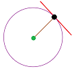
Example. The problem of finding such a line has an easy solution for some specific curves, such as a circle:

Once they realized that the radius and such a line form a $90$ degrees angle, the problem was solved by the ancient Greeks with just ruler and compass. Indeed, one just plot another circle with diameter served by the segment between the point and the center of the original circle... $\square$

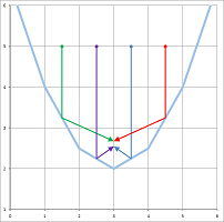
Example (parabola). The history of ancient Greece tells about the famous mathematician Archimedes arranged the shields of the solders along this curve in order to set on fire the ships of the Romans that besieged his city of Syracuse. He used the fact that the light bouncing from a parabolic mirror will all meet at one point called the focus of the parabola. We can confirm that idea but tracing how the light bounces off the secant lines:

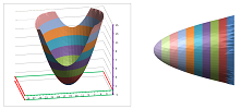
Conversely, a source of light placed at the focus of a parabola will create a beam of parallel rays of light; the fact is used to design cars' headlights:

$\square$

Answering the above question will also answer the questions below.

Example. Of course, a ball would bounce off a wall in the same manner as a beam of light bounces off a mirror. In which direction a billiard ball will bounce off another?

File:Billiard ball.png

$\square$

Example. In which direction a radar signal will bounce off the surface of a plane?

$\square$

Example. Where do the lights of a car traveling on a curvy road point?

$\square$

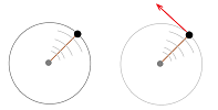
Example. In what direction would a rock released from a sling go (view from above)?

$\square$

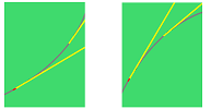
Example. Practically, how do we find the tangent line? As we don't have the luxury of zooming in on a digital image, we draw lines closer and closer to the graph so that the last one touches the graph at that point.

The rule of thumb is that one should expect -- when zoomed out -- only one point in common between the tangent line and the part of the graph of $f$ close to the point $A$. Another way to know that you did it right is to see the tangent line as an edge of a piece of paper; then this piece has to cover none of the (relevant) part of the graph:

There are exceptions; the last image gives you an inflection point with the tangent line cutting the graph in half. $\square$

The analytical method of solving this Tangent Problem is one of the two main motivations (the other one is motion) for the development in this chapter. Geometrically, the starting point is the following. We build a sequence of secant lines: each goes through two points, a fixed point $A=(a,f(a))$ and some variable point $B=(b,f(b))$ with $a\ne b$.

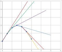
As $B$ is getting closer and closer to $A$, the secants become shorter and shorter, and less and less useful. If we extend these segments into straight lines, we can observe them rotate as they are getting closer and closer to the tangent line. An even better idea is to follow how the slopes -- they are numbers -- of these lines change. We are dealing with a limit!

Location - velocity - acceleration

Recall the case of a broken speedometer from Chapter 1.

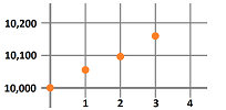
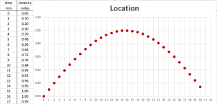
We approached the problem by plotting the location as a function of time:

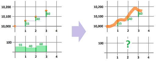
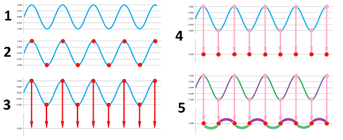
We then found: $$\text{ average velocity }= \frac{\text{ displacement }}{\text{ time }},$$ for each of the time periods (left):

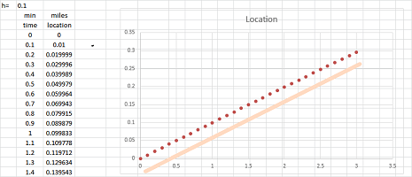
However, what if behind this data is a continuously changing location (right)? With so much information, can we find the “exact” velocity for all of these moments of time?

We now consider a more elaborate version of the problem of incremental motion.

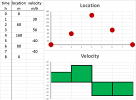
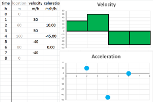
Suppose we drove around while paying attention to the clock and to the mileposts. The result is this simple table with five columns: $$\begin{array}{|l|c|c|c|c|c|} \text{time (hours): }&0&2&4&6&8\\ \hline \text{location (miles): }&0&60&160&80&0 \end{array}$$

What was the velocity over these four periods of time? We estimate it by the familiar “difference quotient” formula (the average rate of change): $$\text{average velocity}=\frac{\text{change of location}}{\text{change of time}}.$$ These are the computations: $$\begin{array}{|l|cccccc|} \text{time (hours): }&0&2&4&6&8\\ \hline \text{location (miles): }&0&60&160&80&0\\ \hline \text{velocity (miles/hour): }&\tfrac{60-0}{2-0}=&30&&&\\ \text{velocity (miles/hour): }&&\tfrac{160-60}{4-2}=&50&&\\ \text{velocity (miles/hour): }&&&\tfrac{80-160}{6-4}=&-40&\\ \text{velocity (miles/hour): }&&&&\tfrac{0-80}{8-6}=&-40\\ \end{array}$$ The four computed values are the average velocities over the following intervals of time: $[0,2]$, $[2,4]$, $[4,6]$, and $[6,8]$, respectively. The result is this table: $$\begin{array}{|l|c|c|c|c|c|} \text{time intervals (hours): }&[0,2]& [2,4]&[4,6]&[6,8]\\ \hline \text{velocity (miles/hour): }&30&50&-40&-40 \end{array}$$ Alternatively, we may choose to assign the four values to the middle points of these intervals, as follows: $$\begin{array}{|l|c|c|c|c|c|} \text{time (hours): }&1&3&5&7\\ \hline \text{velocity (miles/hour): }&30&50&-40&-40 \end{array}$$

This is the summary of what we have found:

This time we also proceed to compute the acceleration. Just as we used the “difference quotient” formula to find the velocity from the location, we now use it to find the acceleration from the velocity: $$\text{average acceleration}=\frac{\text{change of velocity}}{\text{change of time}}.$$ We apply this formula to three periods of time. These are the computations: $$\begin{array}{|l|cccccc|} \text{time intervals (hours): }&[0,2]& [2,4]&[4,6]&[6,8]\\ \text{time (hours): }&1&3&5&7\\ \hline \text{velocity (miles/hour): }&30&50&-40&-40\\ \hline \text{acceleration (miles/hour/hour): }&\tfrac{50-30}{3-1}=&10\\ \text{acceleration (miles/hour/hour): }&&\tfrac{-40-50}{5-3}=&-45\\ \text{acceleration (miles/hour/hour): }&&&\tfrac{-40-(-40)}{7-5}=&0 \end{array}$$ The three computed values are the average accelerations over the following intervals of time: $[0,4]$, $[2,6]$, and $[4,8]$, respectively. This is the result: $$\begin{array}{|l|c|c|c|} \text{time intervals (hours): }&[0,4]&[2,6]&[4,8]\\ \hline \text{acceleration (miles/hour/hour): }&10&-45&0 \end{array}$$ Alternatively, we may choose to assign the three values to the middle points of these intervals, as follows: $$\begin{array}{|l|c|c|c|} \text{time (hours): }&2&4&6\\ \hline \text{acceleration (miles/hour/hour): }&10&-45&0 \end{array}$$

This is the summary of what we have found:

When the location is known for numerous moments of time, we have these sequences:

• $t_n$ for the time,
• $p_n$ for the position,
• $v_n$ for the velocity, and
• $a_n$ for the acceleration.

They are connected by these formulas: $$v_{n+1}=\frac{p_{n+1}-p_n}{t_{n+1}-t_n}\ \text{ and }\ a_{n+1}=\frac{v_{n+1}-v_n}{t_{n+1}-t_n}.$$

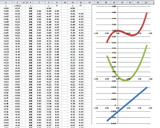
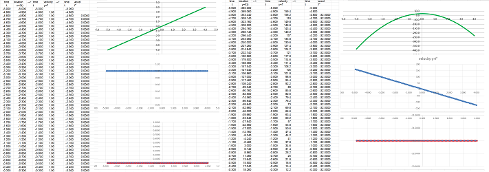
For computations with more extensive, a spreadsheet is used. The two formulas have the same form: $$\texttt{=(RC[-1]-R[-1]C[-1])/(RC2-R[-1]C2).}$$ The formula for the velocity (or the acceleration respectively) refers to the column that contains the location (or velocity respectively) in the numerator and to the column that contains the time in the denominator. Possible data and graphs for these three are shown below:

The second column (velocity) has one fewer data point and the next (acceleration) one fewer yet. However, when zoomed out, the graphs give the impression that the three functions have the same domain.

The story of what happened can be inferred from these graphs:

• 1. the object was moving forward, then stopped for a moment, turned back for a short while, then starting moving forward again;
• 2. the object velocity was forward high, then lower and lower (slower and slower), until it was zero and then changed direction, then forward again, higher and higher (faster and faster);
• 3. the object had negative acceleration (deceleration), which then became positive, and continue to grow.

These formulas will allow us to develop realistic modeling of motion.

However, one of the major reasons to embark on this study is to try to progress from the average velocity presented above to the instantaneous velocity. It's a limit!

The rate of change: the difference quotient of a function

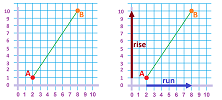
Suppose we know only two values of a function: $$f(x_1)=y_1\ \text{ and }\ f(x_2)=y_2,$$ with $x_1\ne x_2$. Then, what can we say about its rate of change? The answer is given by the slope of the line through these two points on the graph of $y=f(x)$: $$A=(x_1,y_1)\ \text{ and }\ B=(x_2,y_2).$$

It is, of course, rise over the run: $$\text{slope }=\frac{y_2-y_1}{x_2-x_1}=\frac{f(x_2)-f(x_1)}{x_2-x_1}.$$ The numerator, the rise, is the change of $y$, which we will call the difference of $f$, denoted by: $$\Delta f=f(x_2)-f(x_1).$$ The denominator, the run, is the change of $x$, which we will call the increment of $x$, denoted by: $$\Delta x=x_2-x_1.$$ Their ratio, the slope of the line, is the rate of change of $f$, which we will call the difference quotient of $f$, given by: $$\frac{\Delta f}{\Delta x}=\frac{f(x_2)-f(x_1)}{x_2-x_1}.$$

Example. In the above picture, we have:

• the increment of $x$ is $\Delta x=x_2-x_1=8-2=6$;
• the difference of $f$ is $\Delta f=f(x_2)-f(x_1)=10-1=9$;
• the difference quotient of $f$ is $\frac{\Delta f}{\Delta x}=\frac{9}{6}$.

$\square$

If we know only two values of a function (first row) at ends of an interval, we compute the difference quotient along this interval (second row): $$\begin{array}{ccccccc} -&f(x)&---&f(x+\Delta x)&-&\\ -&-\bullet-&\frac{\Delta f}{\Delta x}&-\bullet-&-\\ &x&c&x+\Delta x&&\\ \end{array}$$ As you can see, we subtract the values at the end-points and place the result at the edge.

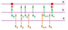
Now, what if a function $y=f(x)$ is known for several values of $x$ within an interval $[a,b]$? We follow the idea of the construction in the beginning of the chapter.

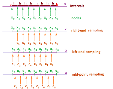
We construct a partition of an interval $[a,b]$. First, we place points on the interval: $$a=x_{0}\le x_{1}\le x_{2}\le ... \le x_{n-1}\le x_{n}=b.$$ As a result, the interval is partitioned into $n$ smaller intervals of possibly different lengths: $$[x_{0},x_{1}],\ [x_{1},x_{2}],\ ... ,\ [x_{n-1},x_{n}],$$ with $x_0=a,\ x_n=b$. The end-points of the intervals, $$x_{0},\ x_{1},\ x_{2},\ ... ,\ x_{n-1},\ x_{n},$$ will be called the nodes of the partition.

We will also use the increments of $x$: $$\Delta x_i = x_i-x_{i-1},\ i=1,2,...,n.$$

In addition to the nodes, the primary nodes, we may also be given the secondary nodes (or sample points) in each interval of the partition: $$ c_{1} \text{ in } [x_{0},x_{1}], \ c_{2} \text{ in } [x_{1},x_{2}],\ ... ,\ c_{n} \text{ in } [x_{n-1},x_{n}].$$

The result is an augmented partition. It is a combination of points: $$ a=x_{0}\le c_1\le x_{1}\le c_2\le x_{2}\le ... \le x_{n-1}\le c_n\le x_{n}=b.$$

In the examples in the introduction and the beginning of this chapter, we had a construction, just like this one, used to compute the velocity from the location when, for example, the location may be represented by a function known only at the nodes of the partition. It was an instance of the above:

• the intervals of the partition were equal in length, and
• the secondary nodes were placed at the end of each interval.

It is called a right-end sampling, for some $h>0$:

• the nodes are $x=a,a+h, a+2h,...$ and
• the secondary nodes are $c=a+h,a+2h,...$.

Next, this is a left-end sampling:

• the nodes are $x=a,a+h, a+2h,...$ and
• the secondary nodes are $c=a,a+h,...$.

Another convenient choice is a mid-point sampling:

• the nodes are $x=a,a+h, a+2h,...$ and
• the secondary nodes are $c=a+h/2,a+3h/2,...$.

The final step is to utilize the secondary nodes as the inputs of the new function:

Definition. Suppose $y=f(x)$ is defined at the nodes $x_k,\ k=0,1,2,...,n$, of a partition. Then the difference of $f$ is a function defined at the secondary nodes of the partition, and denoted, by: $$\Delta f(c_{k})=f(x_{k+1})-f(x_k).$$ Furthermore, the difference quotient of $f$ is defined at the secondary nodes of the partition as this fraction: $$\frac{\Delta f}{\Delta x}(c_{k})=\frac{f(x_{k+1})-f(x_k)}{x_i-x_{i-1}}=\frac{f(x_{k}+\Delta x_k)-f(x_k)}{\Delta x_k},\ k=1,2,...,n.$$

The former concept was defined for sequences in Chapter 1. The latter represents the slopes of the lines that connect the points on the graph of the function.

Note that producing the difference quotient is the very first operation of calculus. Until further operations are introduced, the secondary nodes will remain absolutely arbitrary. For now, this is just bookkeeping...

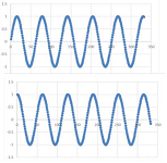
Example. Let's apply the formula to $f(x)=\sin x$. In the first graph below we sample this function every $\Delta x=.1$:

The second graph is the difference quotient. It looks like $y=\cos x$, especially if we shift it a little to the right. $\square$

When a partition is specified, we may omit the subscript for the nodes, $x$, and the secondary nodes, $c$. Then we can use the following simplified notation: $$\Delta f(c)=f(x+\Delta x)-f(x).$$ and $$\frac{\Delta f}{\Delta x}(c)=\frac{f(x+\Delta x)-f(x)}{\Delta x}.$$

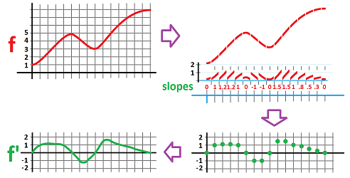
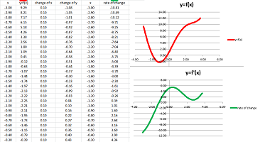
Example. Can we plot $\frac{\Delta f}{\Delta x}$ based on the graph of $f$ only? We do this point by point, i.e., piece by piece. In each of the locations, we extract from the graph a piece that most resembles the tangent line; we simply cut -- using the grid -- a segment of the graph so short that it's almost straight (top right):

The locations of these pieces are irrelevant. We line them up below so that their slopes, the difference quotients of the function, are estimated. This gives us $15$ numbers; these are the approximate values of the derivative $f'$ (bottom right). They are plotted on a new $xy$-plane and then connected into a continuous curve (bottom left). $\square$

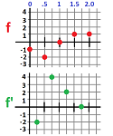
Example. Now we plot $\frac{\Delta f}{\Delta x}$ based on the values of $f$ with the increment of $\Delta x=.5$: $$\begin{array}{r|ccccc} x &0 &.5&1.0&1.5&2.0\\ \hline y=f(x)&-1&-2&0 &1 &1 \end{array}$$ We compute the difference quotient from this data: $$\frac{\Delta f}{\Delta x}(x)= \frac{f(x+\Delta x)-f(x)}{\Delta x}.$$ We do that interval by interval: $$\begin{array}{r|ccccc} [x,x+\Delta x]&[0,.5]&[.5,1.0]&[1.0,1.5]&[1.5,2.0]\\ \hline \Delta f\, (c)=f(x+\Delta x)-f(x)=& -2-(-1)&0-(-2)&1-0&1-1\\ =& -1&2&1&0\\ \frac{\Delta f}{\Delta x}(c)=& -1/.5&2/.5&1/.5&0/.5\\ =& -2&4&2&0\\ \end{array}$$

The results are confirmed by plotting these data points:

These numbers are of course just the slopes of the secant lines. $\square$

Example. We now utilize a spreadsheet to speed up this process. The function is given by a possibly large table of values, with two columns: $x$ and $y=f(x)$. Then, each pair of consecutive values, we compute:

• the increment of $x$,
• the increment of $y$, and
• their ratio, the difference quotient.

The last formula is: $$\texttt{=RC[-2]/RC[-3]}.$$

$\square$

The limit of the difference quotient: the derivative

Suppose we have a function that we can freely sample, i.e., to find its value $y=f(x)$ for any choice of $x$. We would like now make sense of the rate of change of this function in the vicinity of a particular value of $x$.

Example. Let's investigate the rate of change of this function in the vicinity of $x=0$:

These values of $x$ have come from a partition with the original node $a=x_0=0$ and the increment of $x$ chosen to be $\Delta x=1$. The rate of change, i.e., difference quotient of the function for this partition, varies.

Let's now choose a smaller step $\Delta x=.1$:

We can see an almost straight line! In fact, the difference quotient is almost constant. Once this observation has been made, however, we realize that we need just one extra point. In other words, a two-node partition, $a$ and $a+\Delta z$, is sufficient. $\square$

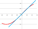
The derivative is the slope of the tangent line. One can estimate this number from a picture by blowing up a small piece surrounding the point and then placing it on a grid:

But what is the tangent line?

To find the tangent line, we only need its slope. We define its slope as the limit of slopes of the cords, called the secant lines, i.e., lines determined by two points on the graph.

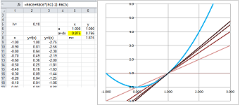
Example. Let's consider $y=x^2$ at $x=1$. Five points are chosen closer and closer to $1$ from the left: $$x=-1,\ 0,\ .5,\ .75,\ ,.875.$$

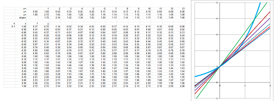
A secant line is drawn through $(1,1)$ and $(x,x^2)$ for these values of $x$. The slopes are evaluated as: $$\frac{x^2-1}{x-1}.$$ The secant lines are shown, and we can see that the last one looks almost tangent to the curve. $\square$

In general, for each $x \neq a$, draw a line through $(a,f(a))$ and $(x,f(x))$: $$\text{slope of the cord } = \frac{\text{rise}}{\text{run}} = \frac{f(x) - f(a)}{x-a}.$$

The difference quotient of a function $f$ at $a$ is defined for each $x\ne a$ to be $$\frac{f(x) - f(a)}{x-a}.$$

Then the slope of the tangent line is the limit of these slopes. As we move $x$ toward $a$, the secant lines turn and approach the tangent line, provided the limit exists.

Definition. The derivative of $f$ at $x$ is defined to be the limit of the difference quotients at $x=a$ as the increment $\Delta x$ is approaching $0$, denoted by: $$\frac{df}{dx}(a)=\lim_{\Delta x \to 0} \frac{\Delta f}{\Delta x}(a)=\lim_{\Delta x \to 0} \frac{f(a+\Delta x) - f(a)}{\Delta x}.$$

Warning: the derivative is not a fraction.

Warning: the derivative is not the limit of $f$, $\lim_{x \to a} f(x)$, but a limit of a new function made from $f$.

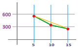
Example. Let's estimate the derivative of a function given by numbers only: $$\begin{array}{l|lll} x&5&10&15\\ \hline y=f(x)&554&344&250 \end{array}$$ What is $\frac{df}{dx}(10)$?

We use the difference quotient, i.e., the slope of a secant line. There are several choices:

We can use the slope of either of the two adjacent secant lines:

• slope of the 1st segment $=\dfrac{344 - 554}{5} = -42$;
• slope of the 2nd segment $=\dfrac{250 - 344}{5} = -18.8$.

We can also use the average of the two.

• average slope $=\dfrac{ -42 + (-18.8)}{2} = \dfrac{-60.8}{2} = -30.4 $.

The last option is to use the two segments as a single interval:

• slope $=\dfrac{250 - 554}{10}=-30.4.$

It's the same number! $\square$

Exercise. Is this a coincidence?

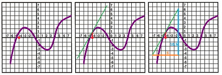
Example. One can estimate the derivative from the graph by using our ability to plot tangent lines. Let's find the derivative at the red point.

• Step 1: plot the tangent line (green);
• Step 2: using the grid, build a right triangle with the segment of the tangent line as its hypotenuse;
• Step 3: find the slope:

$$\text{ slope }=\frac{\text{rise}}{\text{run}} \approx \frac{10.5}{6} = 1.75.$$ To better estimate the slope, draw the triangle as large as possible. $\square$

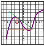
Example. Find the derivative at the point given:

To find the slope, we need the rise. The height of the triangle is $6.5$. However, the only way to justify using the word “rise” while we are going down is to give it a negative value: $$\text{rise }= -6.5.$$ Then the slope and the derivative are also negative: $$\frac{df}{dx}(3)=\frac{-6.5}{9}\approx -7.2.$$ $\square$

Exercise. Find the derivative at the rest of the integer points.

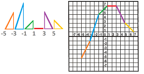
Example. Now we go in the opposite direction: plot the graph based on numerical data. Suppose only these values of the derivative are known: $$\frac{df}{dx}(-5)=2,\ \frac{df}{dx}(-3)=3,\ \frac{df}{dx}(-1)=1,\ \frac{df}{dx}(1)=0,\ \frac{df}{dx}(3)=-2,\ \frac{df}{dx}(5)=-1.$$ Each is the slope of the respective tangent line and, therefore, the rise of this line whenever the run is equal to $1$. We choose the run to be the distance between the points, i.e., $2$. Therefore, the values of the rise are: $$\begin{array}{l|cccccc} x:&-5&-3&-1&1&3&5\\ \hline \text{rise: }&4&6&2&0&-4&-2 \end{array}$$ Then we have six triangles and their hypotenuses are meant to make up rough approximation of the graph of $f$:

We would like to assume that $f$ is continuous! That is why we attach these pieces in such a way that together they make one curve. Note that any vertical shift of this curve will produce an equally correct answer. $\square$

Exercise. Plot the graph of $f$ based on these values of the derivative: $$\frac{df}{dx}(-5)=-1,\ \frac{df}{dx}(-4)=1,\ \frac{df}{dx}(-3)=0,\ \frac{df}{dx}(-2)=2,\ \frac{df}{dx}(-1)=-2,\ \frac{df}{dx}(0)=3.$$

The derivative is the instantaneous rate of change

The derivative is the limit of the difference quotient. We will now use our skills with limits (Chapter 6) to compute more derivatives. For simplicity, we will substitute: $$h=\Delta x.$$

Example. Find the tangent line to $y = x^{2}$ at $(1,1)$.

The slope is the derivative of $y=x^{2}$ at $x=1$. Use $f(x) = x^{2}$, $a =1$ in the definition. $$\begin{aligned} \frac{df}{dx}(a) &= \lim_{x \to a} \frac{f(x) - f(a)}{x - a} \\ & = \lim_{x \to 1} \frac{x^{2} - 1^{2}}{x - 1} \qquad \to \frac{0}{0}? \qquad\begin{array}{|c|}\hline \ \text{ DEAD END }\ \\ \hline\end{array}\\ & = \lim_{x \to 1} \frac{(x-1)(x+1)}{x-1} \\ & = \lim_{x \to 1} ( x + 1 ) \\ & = 1 + 1 \\ &= 2. \quad \text{ That's the slope! } \end{aligned}$$ Then the point-slope form of the line is: $$ y - 1 = 2(x - 1).$$ $\square$

Alternative formula for the derivative. In the formula for the difference quotient, we, instead of concentrating on how $x$ is approaching $a$, look at the (signed) distance $h=x-a$ between them. Then $h\to 0$:

As you can see, the secant lines keep turning, 2nd is closer to the tangent than 1st, etc.

Let's substitute $h = x - a$ into the definition: $$\frac{df}{dx}(a) = \lim_{x \to a} \frac{f(x) - f(a)}{\underbrace{x - a}_{h = x - a}},$$ therefore, $x = a + h$, as follows: $$\frac{df}{dx}(a) = \lim_{h \to 0} \frac{f(a + h) - f(a)}{h}.$$ Thus, what this substitution accomplished is a change of variables in the limit.

Example. This makes computations easier sometimes... Let's consider the last example again: $$f(x) = x^{2}.$$ Compute the difference quotient and its limit: $$\begin{aligned} \frac{df}{dx}(1) &= \lim_{h \to 0} \frac{f(1 + h) - f(1)}{h} \\ & = \lim_{h \to 0} \frac{(1 + h)^{2} - 1^{2}}{h} \\ & = \lim_{h \to 0} \frac{1^{2} + 2h + h - 1}{h} \\ & = \lim_{h \to 0} \frac{2h + h^{2}}{h} \qquad\to \frac{0}{0}? \qquad\begin{array}{|c|}\hline \ \text{ DEAD END }\ \\ \hline\end{array} \\ & = \lim_{h \to 0} (2 + h), \qquad\text{ divide first!}\\ &= 2 + 0 = 2. \end{aligned}$$ $\square$

Example. Find $\frac{df}{dx}(1)$ for $f(x) = \frac{1}{x}$.

$$\begin{aligned} \frac{df}{dx}&= \lim_{h \to 0} \frac{f(1 + h) - f(1)}{h} \qquad \to \frac{0}{0}? \qquad\begin{array}{|c|}\hline \ \text{ DEAD END }\ \\ \hline\end{array} \\ &= \lim_{h \to 0} \frac{\frac{1}{1+h} - \frac{1}{1}}{h} \qquad \to \frac{0}{0}? \qquad\begin{array}{|c|}\hline \ \text{ DEAD END }\ \\ \hline\end{array} \\ &= \lim_{h \to 0} \frac{\frac{1}{1+h} - \frac{1+h}{1+h}}{h} \\ &= \lim_{h \to 0} \left( \frac{1 - (1-h)}{1+h} \cdot \frac{1}{h} \right)\\ &= \lim_{h \to 0} \left(\frac{-h}{1 + h}\cdot \frac{1}{h} \right)\\ &= \lim_{h \to 0} \left(-\frac{1}{1 + h}\right) \\ &= -\frac{1}{1+0} = -1. \end{aligned}$$ At the end, recognizing that this is a rational function continuous on its domain, in order to evaluate the limit, we simply plug in the value. $\square$

Example. Compute the derivative of $f(x)=x^3$ at $a$. Consider $$\frac{x^3-a^3}{x-a}=x^2+xa+x^2\to 3a^3 \text{ as } x\to a.$$ In particular, we conclude that the graph crosses the $x$-axis by touching it:

$\square$

Note that every time we compute the derivative as a (special kind of) limit, we go through the same stages:

• QR $\ \leadsto\ $ indeterminate expression $\ \leadsto\ $ algebra $\ \leadsto$ ...

We should just ignore what we know to be a dead-end and go straight to algebra!

Sometimes algebra is not enough though...

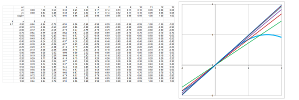
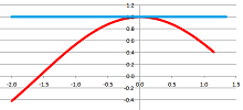
Example. First $f(x)=\sin x$. Then $$\begin{array}{lllll} \frac{\Delta f}{\Delta x}\Bigg|_{x=0}&=\frac{\sin h - \sin 0}{h}\\ &= \frac{\sin h}{h} \\ &\to 1 &\text{ as } h\to 0. \end{array}$$ The last step is simply the following famous trig limit: $$\lim_{x\to 0} \frac{\sin x}{x} =1.$$ The result is confirmed with a spreadsheet:

In other words, the graph of $y=\sin x$ crosses the $y$-axis at $45$ degrees. $\square$

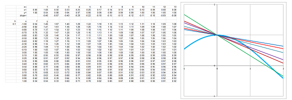
Example. Second, $f(x)=\cos x$. Then $$\begin{array}{lllll} \frac{\Delta f}{\Delta x}\Bigg|_{x=0}&=\frac{\cos h - \cos 0}{h}\\ &= \frac{\cos h -1}{h} \\ &\to 0&\text{ as } h\to 0. \end{array}$$ The last step is simply the other famous trig limit: $$\lim_{x\to 0} \frac{1 - \cos x}{x} = 0.$$ The result is confirmed with a spreadsheet:

In other words, the graph of $y=\cos x$ crosses the $y$-axis horizontally. $\square$

Example. Let $f(x)=e^x$. Then $$\begin{array}{lllll} \frac{\Delta f}{\Delta x}\Bigg|_{x=0}&=\frac{e^h - e^0}{h}\\ &= \frac{e^h-1}{h} \\ &\to 1&\text{ as } h\to 0. \end{array}$$ The last step is simply the following famous limit: $$\lim_{x\to 0} \frac{e^ x-1}{x} =1.$$ The result is confirmed with a spreadsheet:

In other words, the graph of $y=e^x$ crosses the $y$-axis at $45$ degrees. $\square$

The existence of the derivative: differentiability

The process and the methods of finding explicit formulas for the difference quotients and the derivatives for functions given by specific formulas is called differentiation. The former precedes the latter and takes care of all the algebra. The latter required applications of the methods of computing limits presented in Chapter 5.

Warning: “differentiate” has nothing to do with “distinguish” or “tell apart”.

Some limits don't exist. Then, as a limit, the derivative, $$\frac{df}{dx}(a) = \lim_{x \to a} \frac{f(x) - f(a)}{x-a},$$ might not exist either.

Example. To begin with, if a function is undefined at $a$, the numerator is undefined and neither is the derivative at $a$. For example, $\frac{df}{dx}(0)$ doesn't exist for $f(x)=1/x$. $\square$

Suppose now that the function is defined at $x=a$. Then the secant lines are defined but, as $h\to 0$, they might become vertical or simply might not trend toward any particular line.

Example. Let's consider a discontinuous function, $$y=f(x)=\operatorname{sign}(x).$$ We see below how the secant lines become more and more steep, $\text{slope } \to \infty$. So, the limit $\frac{df}{dx}(a)$ is $\infty$:

This how we see this effect in algebra: $$\begin{array}{lll} \frac{df}{dx}(0)&=\lim_{x \to 0} \frac{\operatorname{sign}(x) - \operatorname{sign}(0)}{x - 0}\\ &=\lim_{x \to 0} \frac{\operatorname{sign}(x)}{x}\\ &=\lim_{x \to 0} \frac{1}{|x|}\\ &=\infty. \end{array}$$ This limit does not exist. $\square$

When this limit does exist, what does it tell us? It tells us that there is a tangent line at that location. What does it tell us? It tells us that there is no break in the graph!

Theorem. If the derivative of $f$ exists at $a$, then $f$ is continuous at $a$.

Proof. Let's consider the rise, for $x\ne a$, and rewrite it with the help of the difference quotient as follows: $$f(x) - f(a)=\frac{f(x) - f(a)}{x-a}\cdot (x-a).$$ It's the same function. Let's take the limit of this function as $x\to a$. $$\begin{array}{cccc} \underbrace{\frac{f(x) - f(a)}{x-a}}&\cdot& \underbrace{(x-a)}&=&\underbrace{f(x) - f(a)}\\ \downarrow&&\downarrow&&\downarrow\\ f'(a)&\cdot&0&\Longrightarrow&0 \end{array}$$ So, the limit of the first factor exists and is equal to $f'(a)$ and the limit of the second factor exists and is equal to $0$. Therefore, the Product Rule applies and we have: $$f(x) - f(a)=\frac{f(x) - f(a)}{x-a}\cdot (x-a)\to f'(a)\cdot 0=0.$$ The conclusion, $$\lim_{x \to a} (f(x) - f(a))=0,$$ is rewritten according to the Sum Rule as: $$\lim_{x \to a}f(x) - \lim_{x \to a}f(a)=0.$$ Now, since the limit of a constant function is the constant, $\lim_{x \to a}f(a)=f(a)$, we have: $$\lim_{x \to a}f(x) =f(a).$$ The identity means that $f$ is continuous at $a$. $\blacksquare$

Definition. When the limit of the difference quotient at $a$, $$\lim_{x \to a} \frac{f(x) - f(a)}{x - a},$$ exists, we say that $f$ is differentiable at $a$.

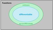
Thus, every differentiable function is also continuous.

Proposition. If $f$ is not continuous at $a$, then $\frac{df}{dx}(a)$ does not exist, i.e., $f$ is not differentiable. However, there are continuous functions that are not differentiable, i.e., the converse isn't true.

Example. If we zoom in on the graph of the absolute value function around $(0,0)$, it won't become a straight line:

The corner won't disappear even after multiple tries. Let's confirm this algebraically and try to compute the derivative of $f(x) = |x|$ at $x=0$. We have: $$\begin{aligned} \frac{df}{dx}(0) &= \lim_{h \to 0} \frac{|0 + h| - |0|}{h} \\ &= \lim_{h \to 0} \frac{|h|}{h}. \\ \end{aligned}$$ Consider: $$\lim_{h \to 0^{-}} \frac{|h|}{h} = \lim_{h \to 0^{-}}\frac{-h}{h} = -1, \qquad \lim_{h \to 0^{+}} \frac{|h|}{h} = \lim_{h \to 0^{+}}\frac{h}{h} = 1.$$ They are not equal, so the limit does not exist. We see this geometrically below:

The secant lines simply follow the line of the graph itself. $\square$

Compare:

• Continuous: there is no break or gap.
• Differentiable: there is no corner or cusp.

As we just saw, when there are two candidates to be a tangent, there is no tangent!

Let's try to use the geometric definition of the derivative -- via secant lines. As we approach $a$ separately from the left and right, they turn, and the end result is...

• Two lines, then $f$ is not differentiable:

• Same line, then $f$ is differentiable:

Algebraically, we verify that the two one-sided limits are equal to each other: $$\lim_{h \to 0^{-}} = \lim_{h \to 0^{+}}.$$

Example. There are functions the graph of which look smooth (no cusps) and yet they are not differentiable:

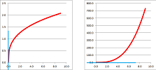
Consider: $$f(x) = \sqrt[3]{x}$$ at $x=0$ (on left).

The limit is infinite: $$\frac{df}{dx}(0) = \infty.$$ How do we know? We conclude that the tangent line at $0$ is vertical from the following fact: $y=\sqrt[3]{x}$ is the inverse of $x=y^3$ (on right) and the derivative of the latter at $0$ is $0$, therefore its tangent line is horizontal at $0$. $\square$

Example. Compute $\frac{df}{dx}(2)$ from the definition for $$f(x) = -x^{2} - x. $$ Definition: $$\frac{df}{dx}(2) = \lim_{h \to 0} \frac{f(2 + h) - f(2)}{h}. $$ To compute the difference quotient, we need to substitute twice. In $f(x) = -x^{2} - x$, we replace $x$ with $2 + h$ and, second, we replace $x$ with $2$: $$f(2 + h) = -(2 + h)^{2} - (2 + h),\ f(2) = -2^{2} - 2.$$ Now, we substitute into the definition: $$\begin{aligned} \frac{df}{dx}(2) &= \lim_{h \to 0} \frac{\left[ -(2 - h)^{2} - (2-h) \right] - \left[ -2^{2} - 2 \right]}{h} \\ &= \lim_{h \to 0} \frac{-4 - 4h - h^{2} - 2 - h + 4 + 2}{h} \\ &= \lim_{h \to 0} \frac{-5h - h^{2}}{h} \\ &= \lim_{h \to 0} (-5 -h ) \\ &= -5 - 0 \\ &= 5. \end{aligned}$$ $\square$

Example. Recall the hypothetical tax code from Chapter 5... If $x$ is the income, then the marginal tax rate is $$f(x) = \begin{cases} 0 & \text{if } &x \le 10000; \\ .10 & \text{if } 10000 < &x \le 20000; \\ .20 & \text{if } 20000 <&x. \end{cases}$$ The tax bill as a function of income is: $$g(x) = \begin{cases} 0 & \text{if } &x \le 10000; \\ .10\cdot (x-10000) & \text{if } 10000 < &x \le 20000; \\ .10\cdot (x-10000)+.20\cdot (x-20000) & \text{if } 20000 <&x. \end{cases}$$

Then $$\frac{dg}{dx}(x)=f(x),$$ except $g$ isn't differentiable, though continuous, for $x=10000$ and $x=20000$. $\square$

The points where the function is differentiable form the domain of the derivative.

The derivative as a function

The difference quotient is a function, defined at the nodes of the partition. What about the derivative?

What if we construct the secant and the tangent lines of a function at all points at the same time? It looks complicated:

To solve the problem, we find, or attempt to find, the derivative -- as the limit of the difference quotient -- at every point $a$ of the domain of $f$. For some of these inputs, we find the value of the derivative $\frac{df}{dx}(a)$, the output. The result is the derivative function! Its domain consists of all points where $f$ is differentiable.

Thus, a new function has been derived from the old! This explains an alternative, more compact, notation for the derivative: $$f'(a)=\frac{df}{dx}(a).$$ What's on the left is called the Lagrange notation and what's on the right the Leibniz notation. The choice between them is a matter of convenience. IF we omit the reference to the input, we are left with the two names of this new function: $$f'=\frac{df}{dx}.$$

We start with the simplest case.

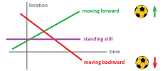
Consider this obvious statement about motion:

• “if I am standing still, my speed is zero”.

If a function $y=f(x)$ represent the position, we can restate this mathematically. We follow what we know about the differences of sequences from Chapter 1: if a function defined at the nodes of a partition of interval $[a,b]$ is constant over the nodes of $[a,b]$, then the function has a zero difference; i.e., $$f(x)=\text{ constant }\ \Longrightarrow\ \Delta f(c)=0.$$ We just divide by $\Delta x$ to prove part (A) of the following.

Theorem (Constant). (A) If a function defined at the nodes of a partition of interval $[a,b]$ is constant over the nodes of $[a,b]$, then the function has a zero difference quotient for all secondary nodes in the partition; i.e., $$f(x)=\text{ constant }\ \Longrightarrow\ \frac{\Delta f}{\Delta x}(c) = 0.$$ (B) If a function is constant on an open interval $I$, then its derivative is zero for all $x$ in $I$; i.e., $$f(x)=\text{ constant }\ \Longrightarrow\ f'(x)=0.$$

Exercise. Prove the theorem.

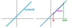
Example (linear). Let's compute the derivative at $x=a$ of a linear function $$f(x)=mx+b.$$ First, the geometry:

Every secant line connects our point of interest, $(a,f(a))$, to another point on the graph, $(a+h,f(a+h))$, where $h=\Delta x$ is the increment of the independent variable. Then, the secant line lies entirely within the straight line that is the graph of $f$. It then has the same slope. Therefore, the derivative must be $m$!

Now, algebra: the difference quotient is independent of location. Indeed: $$\begin{array}{lll} \frac{\Delta f}{\Delta x}(a)&= \frac{f(a + h) - f(a)}{h} &\text{ ...substitute } x=a+h \text{ into the formula of }f,\\ &=\frac{\left[m(a + h)+b\right] - \left[ma+b\right]}{h} &\text{ ...simplify, then }\\ &=\frac{mh}{h} &\text{ ...divide. }\\ &=m&\Longrightarrow\\ \frac{df}{dx}(a)&=\lim_{h \to 0}\frac{\Delta f}{\Delta x}(a)=m. \end{array}$$ The result is a number. However, since is it independent of the chosen $a$, we treat it as a function, a constant function:

$\square$

Based on this example, this is what we conjecture:

• The derivative of a linear function is constant and, conversely, only a constant function can be the derivative of a linear function.

Suppose now that there are two runners; we have a slightly less obvious fact about motion:

• “if the distance between two runners isn't changing, then they run with the same speed”.

It's as if they are holding the two ends of a pole without pulling or pushing.

It is even possible that they speed up and slow down all the time. Once again, for functions $y=f(x)$ and $y=g(x)$ representing their position, we can restate this idea mathematically in order to confirm that our theory makes sense. We follow what we know about the differences of sequences from Chapter 1: if two functions defined at the nodes of a partition of interval $[a,b]$ differ by a constant, then they have the same differences,; i.e., $$f(x) – g(x)=\text{ constant } \ \Longrightarrow\ \Delta f(c) = \Delta g(c).$$ We just divide by $\Delta x$ to prove part (A) of the following.

Theorem (Differentiation). (A) If two functions defined at the nodes of a partition of interval $[a,b]$ differ by a constant, then they have the same the difference quotient; i.e., $$f(x) – g(x)=\text{ constant } \ \Longrightarrow\ \frac{\Delta f}{\Delta x}(c) = \frac{\Delta g}{\Delta x}(c).$$ (B) If two differentiable on open interval $I$ functions differ by a constant, then their derivatives are equal; i.e., $$f(x) – g(x)=\text{ constant } \ \Longrightarrow\ f'(x) = g'(x).$$

Exercise. Prove the theorem.

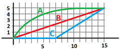
Example. The graph shows the positions of two runners as functions of time. Describe what has happened.

Here's what happened:

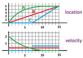
• $A$ starts fast and the slows down, but reaches the finish line first;
• $B$ maintains the same speed;
• $C$ starts late and then runs fast and arrives at the same time as $B$.

We estimate the slopes of the graph. That gives us several values of the velocities. the three graphs are sketched here:

$\square$

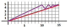
Exercise. Describe what has happened here:

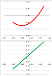
Example (quadratic). What if we pick a quadratic function this time? Let's find $f'=\frac{df}{dx}$ for $f(x) = a x^2 +bx+ c$. $$\begin{array}{lll} \frac{\Delta f}{\Delta x}(x) &= \frac{f(x + h) - f(x)}{h} \\ &= \frac{\left( a[x + h]^2+b[x+h] + c\right) - \left( a x^2+ bx+ c \right)}{h}\\ &= \frac{ ax^2 + 2axh +ah^2+bx+bh + c - a x^2 - bx- c }{h} &\text{ ...the terms without }h \text{ cancel,}\\ &= \frac{2axh +ah^2+bh }{h}&\text{ that's why we can divide by }h!\\ &=2ax +ah+b&\Longrightarrow \\ \frac{df}{dx}(x)&= \lim_{h \to 0}(2ax +ah+b)\\ &=(2ax +ah+b)\Bigg|_{h=0} \\ &= 2ax +b. \end{array}$$ As we see, the difference between the two is a small vertical shift, when $h$ is small enough. For analysis, we match the corresponding parts of the graphs of the function and its derivative (the difference quotient is however what we plot below):

We see how the areas of the graph of $f$ with positive/negative slopes correspond to the area of the graph of $f'=\frac{df}{dx}$ with positive/negative values. $\square$

Based on this example, this is what we conjecture:

• The derivative of a quadratic function is linear and, conversely, only linear functions can be the derivatives of quadratic functions.

Exercise. Prove that the derivative of an odd function is even and the derivative of an even function is odd.

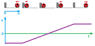
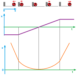
Example (ball ). Suppose we have a rolling ball that hits a wall and then goes back.

This time, the motion is described in terms of its velocity rather than its location! Let's plot the velocity. First, we add the $x$-axis to the picture, with the direction to the right of the wall. Then the velocity of the ball is initially negative!

The velocity at first is constant (and negative) then, as the ball touches the wall and starts to contract, the speed declines. However, this means that the velocity increases! It increases until it reaches $0$ and then it continues to increase as the ball starts to expand. Finally, we the ball leaves the wall, the velocity that has been reached becomes the constant velocity of the motion.

Next, based on the graph of the velocity, we plot the location. Here we use the facts established above:

• a linear location function when the velocity is constant, and
• a quadratic location function when the velocity is linear.

Furthermore, we assume, naturally, that the location is changing continuously:

Whether the graph of location has cusps at the points when the ball touches the wall depends on our assumptions about the qualities of the ball's material. $\square$

Exercise. What if the collision is perfectly rigid? Plot the resulting functions and discuss their continuity and differentiability.

Example (density). Suppose we are given a uniform metal rod:

We define for such a bar: $$\text{average linear density} = \frac{\text{mass}}{\text{length}}.$$

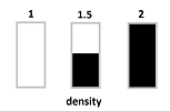
What if the rod isn't uniform, like an alloy? For example, suppose we have two pieces of different metals and we have melt them together (without stirring):

Suppose the densities are $1$ lbs/in and $2$ lbs/in at the ends respectively. Then the density of this alloy will gradually change from $1$ to $2$:

This is the mass function of $x$, the location: $y=m(x)$ is the mass of the rod from $O$ to $x$. Consider how $m$ is changing:

Take a small piece of the rod at location $x$, $\Delta x$ long, and let's call its mass $\Delta m$. Then, for this piece, we have: $$\text{average density} = \frac{\text{mass}}{\text{length}} = \frac{\Delta m}{\Delta x} = \frac{m(x + \Delta x) - m(x)}{\Delta x}.$$ Then we define: $$\text{linear density at }x = \lim_{\Delta x \to 0} \frac{\Delta m}{\Delta x} = m'(x) .$$ $\square$

Warning: Even though $f'$ is derived from $f$, as you can see, there is no way to conjure the whole graph of $f'$ from the look of the graph of $f$... The fact is, a value of $f$ doesn't determine the corresponding value of $f'$ and we shouldn't expect the graph of $f'$ to emerge from shifting the graph of $f$, stretching or shrinking, or flipping, etc.

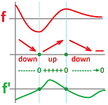
Example. Can we do this more strategically, with fewer points to test?

We first look at the points with a horizontal tangent, i.e., for those $x$'s where $f'(x) = 0$. These will typically separate intervals on which $f' > 0$ or $f' < 0$. To see which one, we look at the directions of the graph of $f$, up or down. We also notice the flattening of the graph on the far right; the result is also flattening of the graph of the derivative -- toward $0$. $\square$

Example (sin). Let's apply this method to the graph of $y=\sin x$. It is easy:

The resulting graph of the derivative looks like that of $y=\cos x$! We will show below that this isn't a coincidence. $\square$

Let's summarize. As $\Delta x$ is approaching zero, there are more and more nodes in the partition and more and more points found on the graph of the function. As a result, there are more and more values of the difference quotient found. Eventually, the former points form the graph of the function and the latter form the graph of its derivative:

What is the meaning of the derivative of a function that represents a transformation?

Let's reexamine the question, what happens to the $x$-axis under such a transformation?

Example (transformations). First a shift: $y=x+k$.

Next, a flip: $y=-x$.

These transformations don't distort the line and are called motions. Next, a stretch: $y=kx$.

A shrink is a stretch with $|k|<1$. Note that a stretch, $y=kx$, is a uniform stretch because the distance between any two points doubles. This ratio is the ratio of the lengths of the corresponding segments in the range and the domain. That's the derivative! With no stretching, the ratio is $1$ unless there is a change of directions (a flip), then its $-1$. The derivative of the collapse, $f(x)=k$, is, of course, $0$.

All the distances between points have become zero as if they have been multiplied by zero. Then, zero is the rate of shrinkage, the derivative. $\square$

We know from Chapter 3 that under a linear polynomial $f(x)=mx+b$ with $m>0$, the distance is increased by a factor of $m$ or decreased by a factor of $m$ when $m<1$. This stretch/shrink factor is the same everywhere. But $m$ is the derivative of $f$!

This is the summary of the functions we have considered:

What are their derivatives? They are respectively: $0,\ 0,\ -1,\ 2$, and $1/2$. We also plot the graphs of these functions below:

Example. Let's consider this function given by its values assuming that the function is a combination of linear patches. We glue -- for the sake of continuity -- these patches together (right): $$\begin{array}{l|lllll} x&0&1&2&3&4&5&6&7&8&9&10\\ \hline y&0&2&5&7&8&8.5&8.5&8&7&4&2\\ \end{array}$$

The derivatives are respectively: $$2,\ 3,\ 2,\ 1,\ 1/2,\ 0,\ -1/2,\ -1,\ -3.$$ $\square$

Exercise. Estimate the derivative from the picture:

In summary, an abstract function $y=f(x)$ has been given three tangible representations and now we also have three tangible interpretations of its derivative: $$\begin{array}{lll} &\text{ function } & \text{ its derivative }\\ \hline 1.&\text{ location } & \text{ velocity }\\ 2.&\text{ graph } & \text{ slope of the tangent line }\\ 3.&\text{ transformation } & \text{ stretch/shrink rate }\\ \end{array}$$

Basic differentiation

Let's consider our current, and then introduce new, notation.

Initially, we deal with one point at a time, $x=a$. First, the difference quotient: $$\frac{\Delta f}{\Delta x}(a)=\frac{f(a+\Delta x) - f(a)}{\Delta x}= \frac{f(x) - f(a)}{x-a},$$ and the derivative: $$\frac{df}{dx}(a) = \lim_{\Delta x \to 0}\frac{\Delta f}{\Delta x}(a).$$

We may also omit any mention of the name of the function in this notation for the difference quotient and the derivative: $$\frac{\Delta y}{\Delta x},\quad \frac{dy}{dx} .$$

In the difference quotient, we use the Greek letter $\Delta$, which stands for “difference”, as follows:

• $\Delta x$ is the change of $x$ (the run), and
• $\Delta y$ is the change of $y$ (the rise).

The former produces the latter with the use of the graph of $y=f(x)$:

The difference quotient is a fraction: $$\frac{\Delta y}{\Delta x}=\frac{\text{change of } y}{\text{change of } x}.$$

Next, in the derivative, we use the letter $d$ that, too, stands for “difference”. The derivative is the limit of a fraction but this doesn't mean that -- in spite of the notation -- it is a fraction too! However, once the derivative is known, at $x=a$, it gives us the slope of the tangent line. Then

• $dx$ is the run, and
• $dy$ is the rise.

The former produces the latter with the use of the graph of the tangent line:

The derivative is a fraction, too: $$\frac{dy}{dx}=\frac{\text{change of } y}{\text{change of } x}.$$

We justify this idea by treating these two quantities, $dx,\ dy$, as a new set of variables.

Definition. Suppose a function $y=f(x)$ is differentiable at $x=a$ and its derivative is $f'(a)$. Then the differential, $dx$, of $x$ and the differential, $dy$, of $y$ are two real variables related to each other by: $$dy=f'(a)\cdot dx.$$

Such an expression is called a differential form to be considered in Chapters 12 and 14.

At every location $a$, the dependence of the two variables is very simple, linear!

Another approach to notation is to present differentiation as a function, a function of functions: $$\frac{\Delta}{\Delta x}(f),\quad \frac{d}{dx}(f).$$

Also convenient sometimes is the notation for evaluating a function at a particular point: $$\frac{\Delta f}{\Delta x}\Bigg|_{x=a},\ \frac{\Delta y}{\Delta x}\Bigg|_{x=a},\ \frac{df}{dx}\Bigg|_{x=a},\ \frac{dy}{dx}\Bigg|_{x=a}.$$ Here both the input and the output are functions!

We may, in fact, omit the names altogether and present only the formula of the function, as follows: $$\begin{array}{lllll} \frac{\Delta}{\Delta x}(3x+5)=3&\ \Longrightarrow\ \frac{\Delta}{\Delta x}(3x+5)\Bigg|_{x=0}&=3\Bigg|_{x=0}&=3;\\ \frac{\Delta}{\Delta x}(-x^2+7)=-2x-2h&\ \Longrightarrow\ \frac{\Delta}{\Delta x}(-x^2+7)\Bigg|_{x=1,\ h=.1}&=-2x-2h\Bigg|_{x=1,\ h=.1}&=-2.2; \end{array}$$ according to the theorems in the last section. This is what we write for the derivatives: $$\begin{array}{lllll} \frac{d}{dx}(-x^2+7)=-2x&\ \Longrightarrow\ \frac{d}{dx}(-x^2+7)\Bigg|_{x=1}&=-2x\Bigg|_{x=1}&=-2;\\ \frac{d}{dx}(3x^2+2x+1)=6x+2&\ \Longrightarrow\ \frac{d}{dx}(3x^2+2x+1)\Bigg|_{x=-1}&=6x+2\Bigg|_{x=-1}&=-4; \end{array}$$ and $$\begin{array}{lllll} (-x^2+7)'=-2x&\ \Longrightarrow\ (-x^2+7)'\Bigg|_{x=1}&=-2x\Bigg|_{x=1}&=-2;\\ (3x^2+2x+1)'=6x+2&\ \Longrightarrow\ (3x^2+2x+1)'\Bigg|_{x=-1}&=6x+2\Bigg|_{x=-1}&=-4. \end{array}$$

Example. This is how we have progressed with the derivative of: $$f(x) = x^2.$$ From a single specific point, to a single unspecified point, to all points at once, a new function! $$\begin{array}{ll|l|l} &a=1&\text{replace }1\text{ with }a&\text{replace }a\text{ with }x\\ \hline &\frac{\Delta f}{\Delta x}(1)= &\frac{\Delta f}{\Delta x}(a)=&\frac{\Delta f}{\Delta x}(x)=&\text{The difference quotient...}\\ &= \frac{f(1 + h) - f(1)}{h} &= \frac{f(a + h) - f(a)}{h}&= \frac{f(x + h) - f(x)}{h}&\text{is written from the definition.}\\ &= \frac{(1 + h)^{2} - 1^{2}}{h}&= \frac{(a + h)^{2} - a^{2}}{h}&= \frac{(x + h)^{2} - x^{2}}{h}&\text{The function is specified.} \\ &= \frac{1^{2} + 2h + h - 1}{h} &= \frac{a^{2} + 2ah + h - a^2}{h} &= \frac{x^{2} + 2xh + h - x^2}{h}&\text{The numerator is expanded.} \\ &= \frac{2h + h^{2}}{h} &= \frac{2ah + h^{2}}{h} &= \frac{2xh + h^{2}}{h} &\text{The terms without }h\text{ are cancelled.}\\ &= 2 + h&= 2a + h&= 2x + h&\text{The numerator is divided by }h.\\ &\to 2 + 0&\to 2a + 0&\to 2x + 0&\text{The limit is evaluated by substitution...}\\ &= 2&= 2a&= 2x&\text{because the function is continuous with respect to }h. \end{array}$$

$\square$

In this section, we will find the derivatives of some important functions. The functions are very different, but the computations will have a lot in common. We need to find the limit of the difference quotient, $$\frac{\Delta f}{\Delta x}=\frac{f(x+h)-f(x)}{h}\ \text{ as } h\to 0.$$ Whenever $f$ is continuous at $x$, the limit of the numerator is $0$. And so is the limit of the denominator! Thus, we will face, every time, the same problem: an indeterminate expression of the type $\frac{0}{0}$. Every time, it is to be resolved, and not by the rules of limits but by algebra! This is the most challenging step:

• we will need factor the numerator in order to cancel $h$ from the difference quotient.

The power functions first. We already know the derivative for the linear and the quadratic powers: $$(x^{1})' = 1, \ (x^{2})' = 2x^{1}.$$ Now cubic: $$f(x)=x^3.$$ We follow the approach in the last section keeping in mind that $x$ is fixed as far as the limit is concerned: $$\begin{array}{ll|lll} \frac{\Delta f}{\Delta x}(x)&= \frac{f(x + h) - f(x)}{h}&\text{The difference quotient is written according to the definition }(h=\Delta x)\\ &= \frac{(x + h)^{3} - x^{3}}{h}&\text{The function is specified.} \\ &= \frac{x^{3} + 3x^2h + 3xh^2+h^3 - x^2}{h}&\text{The numerator is expanded.} \\ &= \frac{3x^2h + 3xh^2+h^3}{h} &\text{The terms without }h\text{ are cancelled.}\\ &= 3x^2 + 3xh+h^2&\text{The numerator is divided by }h. \\ \frac{\Delta f}{\Delta x}(x)&=3x^2 + 3xh+h^2&\text{ This is the simplified difference quotient.} \\ \text{as }h\to 0&\to 3x^2 + 3x\cdot 0+0^2&\text{ The limit is then evaluated by substitution } h=0...\\ &= 3x^2&\text{ because the difference quotient is continuous with respect to }h.& \end{array}$$ We notice something: all the terms disappear except for one or ones that has $h$ in the first power.

The following follows from the binomial formula.

Proposition. The $n$th power, $(x+h)^n$, has $n+1$ terms and the one with $h$ has coefficient equal to $n$: $$(x+h)^n=x^n+nx^{n-1}h+\text{ terms with }h^2,\ h^3,\ ...$$ We will use this fact later.

An alternative approach to factoring relies on the following factoring formula.

Proposition. $$a^n-b^n=(a-b)(a^{n-1}+a^{n-2}b+...+ab^{n-2}+b^{n-1}).$$

We use it as follows ($n=3$): $$\begin{array}{lllll} (x^{3})' & = \lim_{h \to 0}\dfrac{(x + h)^{3} – x^{3}}{h} \\ & = \lim_{h \to 0} \dfrac{(x + h - x)((x + h)^{2} + (x + h)x + x^{2})}{h} \\ & = \lim_{h \to 0} \left[ (x + h)^{2} + (x + h)x + x^{2} \right] \\ & = (x+0)^{2} + (x+0)x + x^{2}\\ & = 3x^{2}. \end{array} $$ We have also discovered a formula for the difference quotient: $$\frac{\Delta}{\Delta x}\left( x^{3}\right)=(x + h)^{2} + (x + h)x + x^{2}.$$

A pattern emerges: $$ \begin{array}{l|ll|ll} n&(x^n)'&\\ \hline 1&(x^1)' & = 1x^0 &1&x&^0 \\ 2&(x^2)' & = 2x^1 &2&x&^1 \\ 3&(x^3)' & = 3x^2 &3&x&^2 \\ ... &... &... &... &... \\ n&(x^n)' & \overset{?}{=} nx^{n-1} &n&x&^{n-1} \end{array} $$

Theorem (Integer Power Formula). Let $n$ be a positive integer. (A) Suppose we have a left-end partition; i.e., the nodes are $x=a,a+h$ and the secondary node is $c=a$. Then the difference quotient of $x^n$ is given by at $c$: $$\begin{array}{ll} \frac{\Delta }{\Delta x}(x^n)=(c + h)^{n-1} + (c + h)^{n-2}c^1 +...+ (c + h)^{1}c^{n-2}+c^{n-1}.\\ \end{array}$$ (B) The derivative of $x^n$ is given by $$\begin{array}{ll} \frac{d}{dx}(x^n)= n x^{n - 1}.\\ \end{array}$$

Proof. The proof relies entirely on either of the two propositions above. $\blacksquare$

Basic differentiation, continued

The Power Formula is now to be tested for other values of $n$.

Example. Let's now try negative powers. Compute: $$\begin{array}{lllll} \left( \dfrac{1}{x} \right)' & = \lim_{h \to 0} \dfrac{\tfrac{1}{x+h}- \tfrac{1}{x}}{h} \\ & = \lim_{h \to 0} \dfrac{\ \tfrac{x - (x + h)}{(x + h)x}\ }{h} \\ & = \lim_{h \to 0} \dfrac{-1}{(x + h)x} & \text{ ...the denominator is continuous for } h<|x|, \\ & = -\dfrac{1}{x^{2}} & \text{...so we substitute } h = 0.\\ \end{array} $$ How does this fit into the above pattern? We rewrite: $$ \dfrac{1}{x} = x^{-1},\ \dfrac{1}{x^{2}} = x^{-2}, ... $$ So, $$ (x^{-1})' = -x^{-2} $$ In other words, we have $n = -1$ and the formula still works. We have also discovered: $$\frac{\Delta }{\Delta x}\left(x^{-1}\right)=\dfrac{-1}{(x + h)x}.$$ $\square$

Example. Next, fractional powers. Compute: $$\begin{array}{lllll} \left( \sqrt{x} \right)' & = \lim_{h \to 0} \frac{\sqrt{x+h}- \sqrt{x}}{h}&\text{ ...indeterminate?} \\ & = \lim_{h \to 0} \frac{\sqrt{x+h}- \sqrt{x}}{h}\cdot \frac{\sqrt{x+h}+ \sqrt{x}}{\sqrt{x+h}+ \sqrt{x}} \\ & = \lim_{h \to 0} \frac{(x+h)- x}{h(\sqrt{x+h}+ \sqrt{x})} \\ & = \lim_{h \to 0} \frac{-1}{\sqrt{x+h}+ \sqrt{x}} &\text{ ...as the function is continuous for }h<|x|, \\ & = \frac{-1}{\sqrt{x+h}+ \sqrt{x}} \Bigg|_{h = 0}&\text{ ...we substitute } h=0 \\ & = \frac{-1}{2\sqrt{x}} . \end{array} $$ How does this fit into the above pattern? We rewrite: $$ \sqrt{x} = x^{1/2},\ \frac{1}{\sqrt{x}} = x^{-1/2}, ... $$ In other words, we have $n = 1/2$ and the formula remains valid. We have also discovered: $$\frac{\Delta}{\Delta x}\left(x^{1/2}\right)=\frac{-1}{\sqrt{x+h}+ \sqrt{x}}.$$ $\square$

This is the general case, to be proven later.

Theorem (Power Formula). For any real number $r\ne 0$, we have: $$(x^r)' = r x^{r - 1}.$$

We would like to find the derivatives of sine and cosine. Before addressing the general case let's recall their derivatives at $x=0$.

Example. We know that the graph of $y=\sin x$ crosses the $y$-axis at $45$ degrees:

This means that the following famous trigonometric limit: $$\lim_{x\to 0} \frac{\sin x}{x} =1,$$ has now a new interpretation: $$(\sin x)'\Bigg|_{x=0}=1.$$

We also know that the graph of $y=\cos x$ crosses the $y$-axis horizontally:

This means that the following famous trig limit: $$\lim_{x\to 0} \frac{1 - \cos x}{x} = 0,$$ has now a new interpretation: $$(\cos x)'\Bigg|_{x=0}=0.$$ $\square$

We now use these results to find the derivative functions of sine and cosine. Remarkably, the derivative of one is the other, up to a sign.

Theorem (Trigonometric Formulas). (A) Suppose we have a mid-point partition; i.e., the nodes are $x=a,a+h$ and the secondary node is $c=a+h/2$. Then the difference quotients of $\sin x$ and $\cos x$ are given by at $c$: $$\begin{array}{llll} \frac{\Delta }{\Delta x}(\sin x)=\frac{ \sin (h/2)}{h/2}\cdot&\cos c;& \frac{\Delta }{\Delta x}(\cos x)=-\frac{ \sin (h/2)}{h/2}\cdot&\sin c.\\ \end{array}$$ (B) The derivatives of $\sin x$ and $\cos x$ are given by $$\begin{array}{llll} \frac{d}{dx}(\sin x)= &\cos x;&\frac{d}{dx}(\cos x)=-&\sin x.\\ \end{array}$$

Proof. First $f(x)=\sin x$. We use the following formula: $$\begin{array}{lllll} \sin u - \sin v = 2 \sin\frac{u-v}{2} \cos\frac{u+v}{2}.\\ \end{array}$$ This formula is the reason why we choose this particular partition. We compute at $c$: $$\begin{array}{lllll} \frac{\Delta f}{\Delta x}&=\frac{\sin (a+h) - \sin (a)}{h}\\ &= \frac{2 \sin (h/2) \cos (a+h/2)}{h} \\ &= \frac{ \sin (h/2)}{h/2}\cdot\cos (a+h/2)&\text{ here } a+h/2 \text{ is exactly the secondary node!}\\ &\to 1\cdot \cos a&\text{ as } h\to 0.\\ &= \cos a. \end{array}$$ The last step is the first famous limit above combined with the continuity of $\cos x$.

The proof of the second identity uses another trig formula, $$\begin{array}{lllll} \cos u - \cos v = -2 \sin \frac{u-v}{2} \sin\frac{u+v}{2}, \end{array}$$ and the other famous limit above. $\blacksquare$

Exercise. Provide a proof of the second formula.

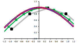
Let's compare the formulas for the difference quotient of $\sin x$ with its derivative: $$\begin{array}{lll} \text{(A)}&\frac{\Delta }{\Delta x}(\sin x)&=\frac{ \sin (h/2)}{h/2}\cdot&\cos (x+h/2);\\ \text{(B)}&\frac{d}{dx}(\sin x)&= &\cos x.\\ \end{array}$$ We know that $$0<\frac{ \sin (h/2)}{h/2}<1,$$ for a small enough $h$. Therefore, the graph of the difference quotient differs from that of the derivative by a vertical shrink and, in addition, a horizontal shift. As $h$ is approaching $0$, the effect of these two operations diminishes; the result is the convergence of the graph of the former to the graph of the latter:

The formulas in the Lagrange notation are as follows: $$(\sin x)'= \cos x,\ (\cos x)'=-\sin x.$$

We will next compute the derivative of the exponential function. Before addressing the general case let's consider its derivative at $x=0$.

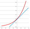
Example. We know that the graph of $y=e^x$ crosses the $y$-axis at $45$ degrees:

This means that the following famous limit: $$\lim_{x\to 0} \frac{e^ x-1}{x} =1,$$ has now a new interpretation: $$(e^ x)'\Bigg|_{x=0}=1.$$ $\square$

We now use this result to find the derivative function of the exponential function. Remarkably, the derivative of the exponential function is itself.

Theorem (Exponential Formula). (A) Suppose we have a left-end partition; i.e., the nodes are $x=a,a+h$ and the secondary node is $c=a$. Then the difference quotient of $e^x$ is given by at $c$: $$\begin{array}{ll} \frac{\Delta }{\Delta x}(e^x)=\frac{ e^h-1}{h}\cdot &e^c.\\ \end{array}$$ (B) The derivative of $e^x$ is given by $$\begin{array}{ll} \frac{d}{dx}(e^x)= &e^x.\\ \end{array}$$

Proof. Let $f(x)=e^x$. We compute at $c$: $$\begin{array}{lllll} \frac{\Delta f}{\Delta x}&=\frac{e^{a+h} - e^a}{h}\\ &= \frac{e^a(e^h-1)}{h} \\ &= e^a\cdot\frac{ e^h-1}{h}&\text{ here } a \text{ is our secondary node!}\\ &\to e^a\cdot 1&\text{ as } h\to 0\\ &=e^a. \end{array}$$ The last step is justified by CMR and the famous limit above. $\blacksquare$

Let's compare the formulas for the difference quotient of $e^x$ and its derivative: $$\begin{array}{rll} \text{(A)}&\frac{\Delta }{\Delta x}(e^x)&=\frac{ e^h-1}{h}\cdot &e^x;\\ \text{(B)}&\frac{d}{dx}(e^x)&= &e^x.\\ \end{array}$$ We know that $$\frac{ e^h-1}{h}>1.$$ Therefore, the graph of the difference quotient differs from that of the derivative by a vertical stretch only. As $h$ is approaching $0$, the stretch diminishes and the graph of the former is approaching the graph of the latter.

The formula in the Lagrange notation is as follows: $$(e^x)'=e^x.$$

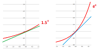
Example. The above computation can be easily applied to the general exponential function, base $b$. Consider, $f(x) = b^{x}, b > 0$. $$ \begin{array}{lllll} (b^{x})' = f'(x) & = \lim_{h \to 0} \frac{f(x + h) – f(x)}{h} \\ & = \lim_{h \to 0} \frac{b^{x + h}- b^{x}}{h} &\to\frac{0}{0}? \text{ ...we need algebra...} \\ & = \lim_{h \to 0} \frac{b^{x} b^{h} - b^{x}}{h} &\text{...use a rule of exponents...} \\ & = \lim_{h \to 0} \frac{b^{x}(b^{h} -1)}{h} & \text{ ...then factor and apply CMR... } \\ & = b^{x} \lim_{h \to 0} \frac{b^{h} - 1}{h} & \text{ ...does this limit exist?} \\ & = b^x \lim_{h \to 0} \frac{b^{0+h} - b^{0}}{h}& \text{ ...it is a familiar one!} \\ &= b^x \cdot (b^x)'\Big|_{x=0}. \end{array}$$ This limit is the slope of the curve at the $y$-intercept, i.e., $f'(0)$, if it exists.

$\square$

Shooting a cannon...

We know that a ball rolling on a horizontal plane will have a constant velocity:

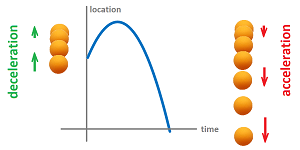
What if the ball is now thrown up in the air? Then the ball goes up, slows down until it stops for an instant, and then accelerates toward the surface. The path “looks like” a parabola:

What if the ball is now thrown under an angle? In this general situation, the ball moves in both vertical and horizontal directions, simultaneously and independently.

The dynamics is very different. In the horizontal direction, as there is no force changing the velocity, the latter remains constant. Meanwhile, the vertical velocity is constantly changed by the gravity. Let's now use these descriptions to represent the motion mathematically.

Earlier in this chapter, we used these difference quotients formulas to find velocity and then the acceleration from the location: $$v_{n}=\frac{\Delta p}{\Delta t}=\frac{p_{n+1}-p_n}{h} \text{ and } a_{n}=\frac{\Delta v}{\Delta t}=\frac{v_{n+1}-v_n}{h},$$ where $h$ is the increment of time. These formulas can now be solved for $p_{n+1}$ and $v_{n+1}$ respectively in order to be able to model location as a function of time: $$v_{n+1}=v_n+ha_n \text{ and } p_{n+1}=p_n+hv_n.$$ These are recursive formulas.

This time we have two such sequences, for horizontal and vertical.

We construct the Cartesian coordinate system in the most convenient way:

• the $x$-axis is horizontal,
• the $y$-axis is vertical,
• the origin is at the base of the hill just under the cannon.

As you can see, we abandon the familiar $y=f(x)$ setup. We have three variables:

• $t$ is time;
• $x$ is the horizontal dimension, the depth;
• $y$ is the vertical dimension, the height.

Either of the two spatial variables depends on the temporal variable.

Meanwhile, the path of the ball will appear to an observer as a curve in the (vertical) $xy$-plane:

Historically, one of the very first applications of calculus was in ballistics. Before calculus, one had to resort to trial and error and watching where the cannonballs were landing. A well-designed test may provide one with a table (i.e., a function) that gives the shot length for each angle of the barrel. However, such a reference table may prove useless when one to shoot from an elevated position, or at an elevated target, or over an obstacle.

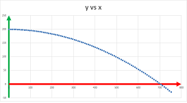
Problem: From a $200$ feet elevation, a cannon is fired horizontally at $200$ feet per second. How far will the cannonball go?

We have these sequences: $$\begin{array}{l|l|l} &\text{ horizontal }&\text{ vertical }\\ \hline \text{ position }&x_n &y_n\\ \text{ velocity }&v_n=\frac{x_{n+1}-x_n}{h} &u_n=\frac{y_{n+1}-y_n}{h}\\ \text{ acceleration }&a_n=\frac{v_{n+1}-v_n}{h} &b_n=\frac{u_{n+1}-u_n}{h}\\ \end{array}$$

Now, from the point of modelling, the derivation should go in the opposite direction. We go in reverse: the velocity and then the location from the acceleration. When we solve the above formulas, we end up with recursive formulas: $$\begin{array}{l|l|l} &\text{ horizontal }&\text{ vertical }\\ \hline \text{ acceleration }&a_n &b_n\\ \text{ velocity }&v_{n+1}=v_n+ha_n&u_{n+1}=u_n+hb_n\\ \text{ position }&x_{n+1}=x_n+hv_n&y_{n+1}=y_n+hu_n\\ \end{array}$$

Now the specific case of free fall, there is just one force, the gravity. Therefore, the horizontal acceleration is zero and the vertical acceleration is constant (feet per second squared): $$a=0,\ b=-32.$$

Next, we acquire the initial conditions:

• the initial location is: $x_0=0$ and $y_0=200$;
• the initial velocity is: $v_0=200$ and $u_0=0$.

We use the formulas to evaluate the location every $.1$ second. This is what the path looks like:

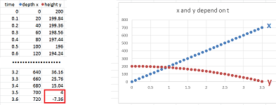
Example (how far). To find when and where the ball hits the ground, we scroll down to find the row with $y$ close to $0$.

It happens sometime between $t=3.5$ and $t=3.6$ seconds, say $t_1=3.55$ seconds. Second, the values of $x$ at the time is between $x=700$ and $x=720$ feet, say, $x_1=710$ feet. We also plot the graphs of $x$ and $y$ as functions of $t$ on the right. $\square$

With the spreadsheet, we can ask and answer a variety of questions about such motion. But first, let's introduce the angle of the cannon into the model.

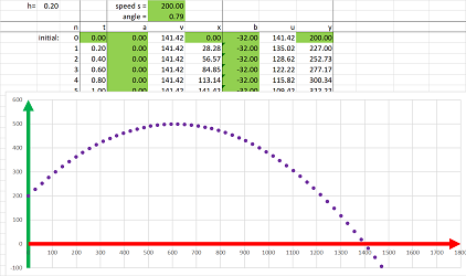
The velocity of $200$ feet per second we have been using is the “muzzle velocity”, i.e., the speed, $s$, with which the cannonball leaves the muzzle -- no matter what the angle, $\alpha$, is. That's where the initial horizontal and the vertical velocities come from: $$v_0=s\cos \alpha,\ u_0=s\sin \alpha.$$

We can enter freely the data for the following (highlighted in green):

• the speed,
• the angle,
• the initial conditions, and
• the accelerations.

The rest is computed according to the formulas above.

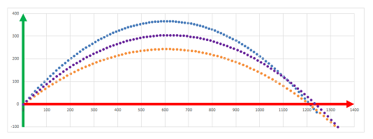
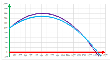
Example (longest). Is it really true that $45$ degree is the best angle to shoot for longer distance? We just try to shoot with an angle just above and just below:

It appears that the one in the middle is the best, but we can't prove this with just the numerical methods... Now, what if we try to shoot from a hill again, say, $500$ feet high?

It's not the best anymore! $\square$

Exercise. Show that the best shot will become more and more flat as the elevation grows.

Example (variable gravity). What happens if the gravity suddenly disappears? In the column for the vertical acceleration, we just replace $-32$ with $0$ after a few rows:

The cannonball flies off on a tangent. $\square$

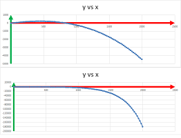
Example (variable gravity). What happens if the gravity starts to increase? We try to increase the down acceleration $1$ foot per second squared per second:

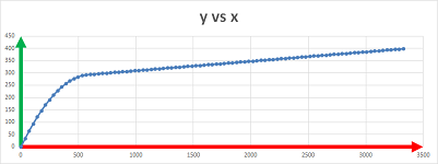
The trajectory looks steeper and steeper, but is there a vertical asymptote? We can't answer with just the numerical methods... $\square$

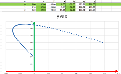
Example (horizontal gravity). What happens if the gravity is horizontal? What if there is both vertical and horizontal gravity? We just modify the acceleration columns accordingly:

$\square$

Exercise. Explain the results in the last example.

In spite of these numerous examples, we can only do one at a time! The conclusions we draw are also specific to these situations. This why we now consider the continuous case, i.e., we take the limit of everything above: $$h=\Delta x\to 0.$$

Instead of six sequences, we have this time these six functions of time:

• $x$ is the depth, the horizontal location;
• $v=x'$ is the horizontal velocity;
• $a=v'$ is the horizontal acceleration;
• $y$ is the height, the vertical location;
• $u=y'$ is the vertical velocity;
• $b=u'$ is the vertical acceleration.

Now the specific case of free fall: $$a=0,\ b=-g.$$ Here $g$ is the gravitational constant: $$g=32 \text{ ft} / \text{sec}^2.$$

We have learned in this chapter that

• the derivative of a quadratic polynomial is linear, and
• the derivative of a linear polynomial is constant.

We will show in Chapter 9 that, conversely,

• the only function the derivative of which is linear is a quadratic polynomial, and
• the only function the derivative of which is constant is a linear polynomial.

We conclude that

• $x=x(t)$ is linear and
• $y=y(t)$ is quadratic.

What makes these specific are the initial conditions:

• $x_0$ is the initial depth, $x_0=x(0)$,
• $v_0$ is the initial horizontal component of velocity, $v(0)=\frac{dx}{dt}\Big|_{t=0}$,
• $y_0$ is the initial height, $y_0=y(0)$, and
• $u_0$ is the initial vertical component of velocity, $u(0)=\frac{dy}{dt}\Big|_{t=0}$.

Therefore, we have $$\begin{cases} x&=x_0&+v_0t,\\ y&=y_0&+u_0t&-\tfrac{1}{2}gt^2, \end{cases}$$

These two equations allow us to solve a variety of problems about motion. We carry this out for $x$ and $y$ separately and the results are shown in the spreadsheet:

Let's revisit the problem about a specific shot we solved numerically. Our equations become: $$\begin{cases} x&=&200t,\\ y&=200&&-16t^2. \end{cases}$$

Example (how far). Now, analytically, the height at the end is $y_0$, so to find when it happened, we set $y=0$, or $$200-16t^2=0,$$ and solve for $t$. Then, the time of landing is: $$t_1=\sqrt{\frac{200}{16}}=\frac{5\sqrt{2}}{2}.$$ To find where it happened, we substitute this value of $t$ into $x$; the location is: $$x_1=200t_1=200\frac{5\sqrt{2}}{2}\approx 707.$$ The result matches our estimate! $\square$

We will prove in Chapter 10 that the longest distance is achieved when shot at $45$ degrees.

Example (accuracy). From the practical point of view, no shot is perfectly accurate. Even when the mathematics is seen as perfect, our limited knowledge of the many parameters that affect the accuracy of our shot will make us under- or overestimate the final location of the cannonball. Let's take just one: the accuracy of our measurement of the height of the hill. If the height, $H$, varies, then so will the placement, $D$, of the shot. The good news is that the smaller error in the former will lead to a smaller error in the latter!

In fact, we can achieve any required degree of accuracy, $\varepsilon$, of our shot if we can ensure a sufficient accuracy, $\delta$, of the measurement of the height of the hill. In other words, the dependence of $D$ on $H$ is continuous. $\square$

Theorem. The distance of the shot depends continuously on the initial elevation.

Exercise. Prove this theorem algebraically.

Exercise. What if instead of target shooting this was a game of tennis?

Exercise. Prove that the distance of the shot depends continuously on the initial angle.

It so happens that the path is the graph of $y$ is a function of $x$! In that case, this dependence can also be found by substitution of $t$ as a function of $x$ into $y(t)$.

Is the path a parabola? It looks like one when plotted point by point (as above), but let's do the algebra now. By substitution, whenever $v_0\ne 0$, we have: $$x=x_0+v_0t\ \Longrightarrow\ t=(x-x_0)/v_0\ \Longrightarrow\ y=y_0+\tfrac{u_0}{v_0}(x-x_0)-\tfrac{g}{2v^2_0}(x-x_0)^2. $$ This is a quadratic function! We have proven it:

• the trajectory of the cannonball is a parabola.

That's why the path traced in the sky is curved this way...

Exercise. What is the path when $v_0=0$?

Exercise. Show that the coefficient $\tfrac{u}{v}$ is the tangent of the angle of the shot.