This site is being phased out.
Manifolds model a curved universe
Redirect to:
Our goal is calculus in the curved universe.
In this curved environment we want to be able to compute: tangents, lengths, areas, volumes, etc.
Contents
Curved universe
The universe is curved, but how do we know?
Observations show that using the Euclidean geometry for wrong scale doesn't work.
In other words, locally, the universe is like ${\bf R}^3$, but not globally.
We can see this in several ways...
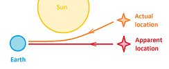
Experiment 1: with light from a star passing the sun and deviating from straight line.
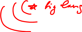
Experiment: interference of light with itself (see elsewhere).
Curved Earth
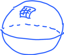
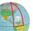
A simpler setting is ${\bf R}^2$. We can consider the Earth as a model.
Here's a fun idea:
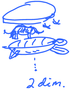
A flat Earth rests on the backs of three elephants who stand on the back of a enormous turtle (and then turtles all the way down...).
It is 2-dimensional!
How do we know it's not flat?
There have been a few experiments...
Experiment 1: Eratosthenes', compare the lengths of shadows of the same object at two different locations $\longrightarrow$ geometry.
Experiment 2: Magellan's, will I come back? $\longrightarrow$ topology.
Experiment 3: Gauss', check that sum of angles of triangle $= 180^o$ on three mountain peaks $\longrightarrow$ geometry
In fact, $> 180^o$! Why? Consider $2$ opposite meridians $+$ equator $= 360^o$.
Curved roads
Even simpler than the 2-dimensional Earth, what about ${\bf R}^1$?
What's locally like ${\bf R}^1$ but not globally?
Roads behave like that, when there are no intersections...
We are talking about curves.
Specifically, one can concentrate on parametric curves: $$f \colon {\rm time} \rightarrow {\rm space}$$ The space may be 3d or 2d. The image of $f$ is also called a parametric curve and it is $1$-dimensional "generically". They are usually required to be continuous or even differentiable.
In that case, is the image of $f$ locally ${\bf R}^1$?
Not generally.
Examples...
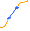
Half of ${\bf R}^1$:
There is a boundary...
What if we require the curve to be "closed", i.e., $f(a) = f(b)$?
Other problems?
Not like ${\bf R}^1$:
We need to require the curve to have no self-intersections, i.e., $f(t) \neq f(s)$ for all $a < s < t < b$.
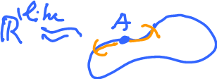
To summarize, we require $f$ to be one-to-one, except possibly for $a,b$. In that case, the image is like ${\bf R}^1$ around any $f(x)$, $t \in (a,b)$. Formally, this is called a "homeomorphic image" of $R$, or an embedding:
Here: $A = f(a) = f(b)$.
Definition: If every point $a \in C$ has an open (in $C$) set $U$, $a \in U$, homeomorphic to ${\bf R}^1$, then $C$ is called a $1$-manifold.
For simplicity, we assume $C \subset {\bf R}^N$.
In that case, $U$ can be chosen simply as $U=C \cap $(open in ${\bf R}^N)$. This means that there is a function $p \colon {\bf R} \rightarrow U$, which is
- one-to-one,
- onto,
- continuous, and
- the inverse $p^{-1}$ continuous too
(aka "homeomorphism").
Example:
Differential forms on curves
Now, what do differential forms look like when they are defined on manifold?
Let's consider $1$-forms on curves -- instead of ${\bf R}$?
Recall $y = f(x)$ is a $0$-form and $dy=f'(x)dx$ is a $1$-form.
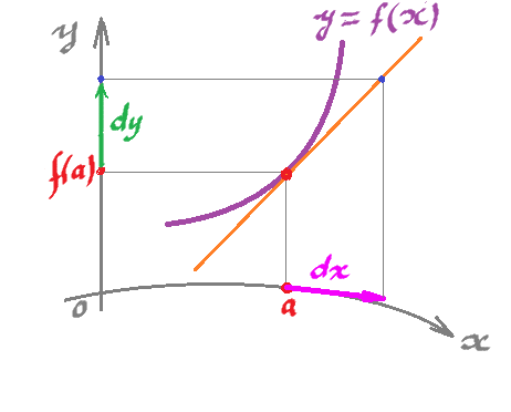
Let's review some calc 1. Where does this equation, $dy = f'(a)dx$, come from?
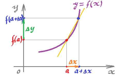
Recall that $f'(a)$ represents the slope of the tangent. But it comes as a limit of slopes of secant lines:
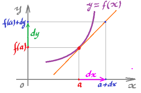
The average change of $y$ is found as: $$\Delta y = f(a+ \Delta x) - f(a)$$ by using the graph of $f$. But for $dy$, we use the tangent line instead:
With $a$ fixed, the derivative is a linear function: $$f'(a):dx \longmapsto dy,$$ $$f'(a):x-axis \longrightarrow y-axis,$$ computed simply as multiplication by number $f'(a)$.
Now, one can think of these variables as vectors in the following vector spaces:
- $dx \in {\bf R}$, its zero is at $a$.
- $dy \in {\bf R}$, its zero is at $f(a)$.
This seemingly awkward point of view becomes very productive once we ask this question:
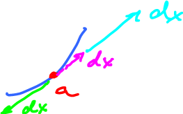
- What if the $x$-axis is curved? Where would this vector $dx$ come from?
Compare:
- We have used $f \colon \stackrel{x}{ {\bf R} } \rightarrow \stackrel{y}{ {\bf R} }$.
- Now we deal with $f \colon \stackrel{x}{ C } \rightarrow \stackrel{y}{ {\bf R} }$, where $C$ is a curve in ${\bf R}^2$.
The setup would look like this:
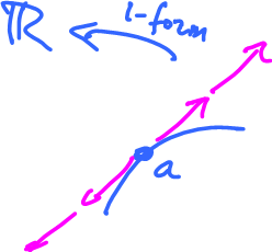
This suggests that we should choose for $dx$ tangent vectors to the curve $C$ at $a$.
It is important to note here that even though $dx$ is still an element of a 1-dimensional vector space, just as in the Euclidean setup, this vector space varies from point to point. Together these lines form the tangent bundle of $C$.
We have our function defined now on a curve $f \colon C \rightarrow {\bf R}$. Here $C$ is a parametric curve given by a differentiable function $p \colon [a,b] \rightarrow C$ with an extra condition: $p' \ne 0$.
Now, we know that the tangent vectors, $dx$, to this curve at this point are to be found as multiples of $p'(t_0)$ if $p(t_0)=a$.
Since $y=f(x)$, we have $y = f(p(t))$ and $$y'(t) = f'(p(t))p'(t).$$
At this point $a = p(t_0)$, we have $$y'(t_0) = f'(a)p'(t_0).$$
So, $f'(a)$ transforms vectors tangent to $C$ at $a$, i.e., $dx$, to those tangent to the $y$-axis at $f(a)$, i.e., $dy$.
To summarize, $dy = Adx$, where $A=f'(a)$ is a linear operator.
Definition. A $1$-form on a curve $C$ is a function linear on the vectors tangent to $C$ at $a$, for each $a$.
The domain of this $1$-form is the tangent bundle of $C$.
Examples of curves and surfaces
$1$-manifolds, just a few:
- closed finite:
- open finite:
- open infinite:
- and their disjoint unions.
They are easy to parametrize:
- $f \colon [a,b] \rightarrow {\bf R}^N$,
- $f \colon (a,b) \rightarrow {\bf R}^N$, and
- $f \colon {\bf R} \rightarrow {\bf R}^N$.
What about surfaces?
They are $2$-manifolds:
- Sphere (parametrization by the spherical coordinates):
- Torus (can be parametrized with a single function):
Can we parametrize it with a single function?
It is difficult.
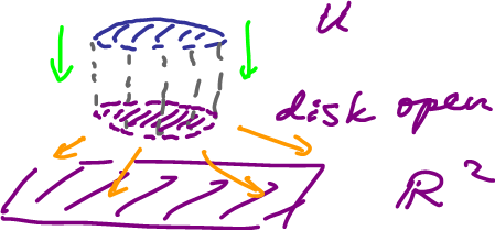
Definition: A $2$-manifold $S$ is a subset of ${\bf R}^N$ such that every point $a \in S$ has an open set $U$ such that $a \in U$ and $U$ is homeomorphic to ${\bf R}^2$.
Note: "homeomorphic to ${\bf R}^2$ can be replaced with "homeomorphic to an open disk".
Manifolds
Similarly we treat the general case...
Definition: An $n$-manifold is a subset $M$ of ${\bf R}^N$, such that for every point $a \in M$ there is an open subset $U$ of $M$ (called a "patch"), $a \in U$, homeomorphic to ${\bf R}^n$.
"Open subset of $M$" simply means that it's the intersection of an open subset of ${\bf R}^N$ with $M$.
Equivalently,
- $p \colon {\bf R}^n \rightarrow U$ is a homeomorphism, or
- $q \colon B^n(0,1) \rightarrow U$ is a homeomorphism,
where $B^n(0,1)$ is the open unit ball in dimension $n$.
If $p \in C^k$, then $M$ is called a $C^k$-manifold.
These are the simplest examples....
Example: $0$-manifolds
- point,
- $n$ points,
- ${\bf N} \subset {\bf R}^1$,
- $\{0\} \cup \{\frac{1}{n} \colon n=1,2,\ldots\}$ is not (exercise),
- $\{\frac{1}{n} \colon n=1,2,\ldots\}$ is.
Example: $N$-manifolds in ${\bf R}^N$
- ${\bf R}^N$,
- $B^N(0,1)$,
- open sets in ${\bf R}^N$.
Example: $n$-manifolds in ${\bf R}^N$, for $n < N$
- $n$-dimensional affine subspaces.
What's not here?
- $[a,b]$ not a $1$-manifold, $N=1$.
It's a closed piece of the line.
Example:
All open sets in the interval look like this (the pink).
Here:
- $V \not\simeq (0,1)$ or ${\bf R}$,
- $V \simeq (0,1]$ half-open,
- $V \simeq {\bf R}_+$.
Similarly,
- ${\bf R}_+ = \{ x \colon x \geq 0\}$, half-line;
- ${\bf R}^2_+ = \{(x,y) \colon y \geq 0\}$, half-space, closed;
- ${\bf R}^n_+ = \{(x_1,\ldots,x_n) \colon x_n \geq 0\}$ half-space, closed.
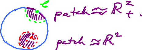
Definition: A subset $M$ of ${\bf R}^n$ is an $n$-manifold with boundary (which might be $\emptyset$) if for every point $a \in M$, there is a patch $U$ such that $a \in U$:
- $p \colon {\bf R}^n \rightarrow U$ is a homeomorphism, or
- $p \colon {\bf R}^n_+ \rightarrow U$ is a homeomorphism.
These patches are also called "coordinate patches" as they create a local coordinate system for $M$.
Example:
Example: In ${\bf R}^N$, $n$-manifolds with non-empty boundary:
- disk,
- square,
- cylinder,
- non-hollow pyramid,
- closed $3$-ball,
- closed $n$-ball,
- ray,
- Mobius strip, etc
We will exclude: ray, open set, etc and concentrate on compact manifolds, i.e., closed and bounded subsets of ${\bf R}^N$.
