This site is being phased out.
Applications of integral calculus
Contents
- 1 The area between two graphs
- 2 The linear density and the mass
- 3 The center of mass
- 4 The radial density and the mass
- 5 The flow velocity and the flux
- 6 The force and the work
- 7 The total and the average value of a function
- 8 Numerical integration
- 9 Lengths of curves
- 10 The coordinate system for dimension $3$
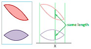
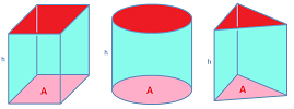
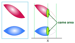
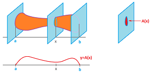
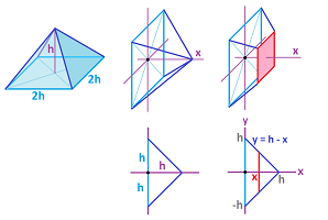
- 11 Volumes via cross-sections
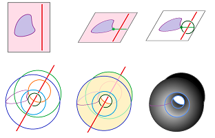
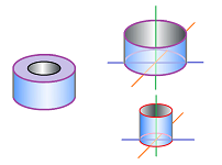
- 12 Volumes of solids of revolution
The area between two graphs
There are two main ways to enter differential calculus: through the study of geometry -- finding secant and tangent lines of curves -- and through the study of motion -- finding velocity and acceleration from location. Similarly, there are two main ways to enter integral calculus: through the study of geometry -- finding areas under curves -- and through the study of motion -- finding location from velocity and acceleration. These are two very distinct examples of recognizing Riemann sums. Throughout this chapter, we will carry out this key step in a variety of situations. But we will start with something familiar...
Example (area of circle). In Chapter 12, we confirmed that the area of a circle of radius $r$ is $A = \pi r^{2}$ with nothing but a spreadsheet. The solution, however, wasn't fully satisfactory because we relied on the symmetry of the circle to compute the area of its half so that the area of the whole circle is then twice this number. This is too limiting... Let's start over.
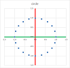
There are two functions this time, for the top and the bottom of the circle: $$f(x)=\sqrt{1-x^2}\ \text{ and }\ g(x)=-\sqrt{1-x^2},\quad -1\le x\le 1.$$ With the formulas: $$\texttt{=SQRT(1-RC[-2]^2)}\ \text{ and }\ \texttt{=-SQRT(1-RC[-2]^2)},$$ we plot both:
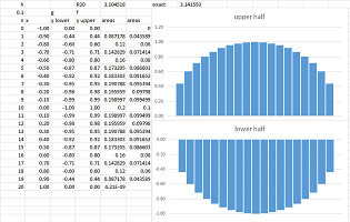
We let the values of $x$ run from $-1$ to $1$ every $.1$ and covered, best we can, this circle with vertical bars based on these segments. Then the area of the circle is approximated by the sum of the areas of the bars: we add a column of the widths of the bars, multiply them by the heights, place the result in the last column, and finally add all entries in this column.
The height the one at $x$ is $f(x)-g(x)$ and its area is $(f(x)-g(x))\cdot .1$. We compute these in the next column and then add them: $$\text{approximate area of the circle}= 3.1....$$ It is close to the theoretical result we established in the last chapter: $$\text{exact area of the circle}= \pi=3.14159...$$ Of course, we realize that we could produce the same result if we take the data from the first spreadsheet, $\sum_i f(c_i)\cdot.1$, and them subtract the data for the new function, $\sum_i g(c_i)\cdot.1$. Furthermore, we have $$\sum_i f(c_i).1+\sum_i g(c_i)\cdot.1=\sum_i (f(c_i)- g(c_i))\cdot.1.$$ $\square$
The common sense about how the (unsigned) lengths of intervals behave is that the length of the union of two intervals is the sum of the two lengths minus the lengths of the intersection: $$\text{ length of }P\cup Q=\text{ length of } P+\text{ length of } Q-\text{ length of } P\cap Q.$$
It is called the additivity of the length. The last term disappears when there is no overlap or it is just a point.
If we build rectangles on top of these intervals, we are in a similar situation -- for the (unsigned) areas:
In other words, the area of the union of two regions is the sum of the two areas minus the area of the intersection: $$\text{ area of }P\cup Q=\text{ area of } P+\text{ area of } Q-\text{ area of } P\cap Q.$$ It is called the additivity of the area. The last term disappears when there is no overlap or it is just a curve.
However, our understanding of areas is limited to those of regions under graphs of functions. Even then, the additivity of the areas of those regions has been only demonstrated for the special case when such a region is cut by a vertical line: $$\int _a^bf\, dx+\int _b^cf\, dx=\int _a^cf\, dx.$$ This case is illustrated below (the line is $x=b$):
What if the region under the graph is cut by another graph?
This gives us the area of the region between the graphs:
The integral interpretation is easy to see; if $f(x)\ge g(x)$ for all $x$ in $[a,b]$, then: $$P=R-Q=\int _a^bf\, dx-\int _a^b g\, dx=\int _a^b(f-g)\, dx.$$ We have assumed the additivity of the areas and used the Sum Rule for the definite integral.
However, every term in the formula is the area under the graph. In order to justify the additivity for the areas between the graphs, we need to start from scratch. Back to approximations...
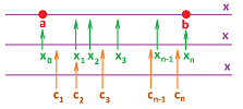
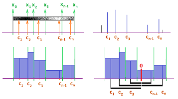
We start, as before, with a partition of the interval $[a,b]$ into $n$ intervals of possibly different lengths: $$ [x_{0},x_{1}],\ [x_{1},x_{2}],\ ... ,\ [x_{n-1},x_{n}],$$ with $x_0=a,\ x_n=b$.
The nodes of $P$ are: $$x_{0}< x_{1}< x_{2}< ... < x_{n-1}< x_{n}.$$ The lengths of the intervals are: $$\Delta x_i = x_i-x_{i-1},\ i=1,2,...,n.$$ The secondary nodes of $P$ are: $$ c_{1} \text{ in } [x_{0},x_{1}], \ c_{2} \text{ in } [x_{1},x_{2}],\ ... ,\ c_{n} \text{ in } [x_{n-1},x_{n}].$$
We now approximate the area between the graphs with rectangles with these widths:
Let's take a look at the $i$th rectangle. Its width is, as before, $\Delta x_i$. Now, its top is $f(c_{i})$ and the bottom is $g(c_{i})$. Therefore, its height is $f(c_{i})-g(c_{i})$. Then, its area is $(f(c_{i})-g(c_{i})) \Delta x_2$. Hence, the total area of the rectangles is: $$(f(c_{1})-g(c_{1}))\Delta x_1 + (f(c_{2})-g(c_{2})) \Delta x_2 + ... + (f(c_{n})-g(c_{n}))\Delta x_n. $$ The key step is the following. We recognize this expression as the Riemann sum of a new function, $f-g$: $$\sum_{[a,b]} (f-g) \, \Delta x= \underbrace{\sum_{i=1}^{n} (f-g)(c_{i})\Delta x_i}_{\text{areas of the rectangles}}. $$ The rectangles we started with are shown on the left and the Riemann sum of the difference on the right:
We can still go back and explain the Riemann sum of the new function in terms of areas. It's as if the rectangles are first aligned with $y=f(x)$, then cut from below with $y=g(x)$, suspended in the air, and then dropped on the $x$-axis, like this:
We see the area under the graph of $f-g$.
Definition. Suppose $f$ and $g$ are two functions defined on interval $[a,b]$ with $f(x)\ge g(x)$ for all $x$ in $[a,b]$. Then the area between the graphs of these functions over interval $[a,b]$ is defined to be the limit of a sequence of the Riemann sums of their difference with the mesh of their augmented partitions $P_k$ approaching $0$ as $k\to \infty$, when all these limits exist and are all equal to each other: $$\text{Area between the graphs of } f,g = \lim_{k \to \infty} \sum_{[a,b]}(f-g) \, \Delta x.$$
Exercise. If $f$ and $g$ represent the velocities of two objects, what does the area represent?
Theorem. Suppose $f$ and $g$ are two functions defined on interval $[a,b]$ with $f(x)\ge g(x)$ for all $x$ in $[a,b]$. If $f-g$ is integrable, then the area between the graphs of $f$ and $g$ is equal to $$\int_a^b(f-g)\, dx.$$
We have a variety of regions we used to be unable to compute.
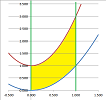
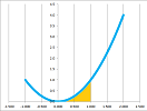
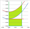
Example (parabolas). Evaluate the area of the region is bounded by the parabolas $y=x^2$ and $y=2x^2+1$ between $x=0$ and $x=1$. It is clear that $g(x)=x^2$ and $f(x)=2x^2+1$, as well as that $a=0$ and $b=1$. The functions are continuous and, therefore, integrable. Before we apply the formula, we just need to confirm that the graph of $f$ is above the graph of $g$:
For every $x$ between $0$ and $1$, we have $x^2<2x^2 +1$ because $0<x^2 +1$. Thus, $$\text{Area }=\int_a^b(f-g)\, dx=\int_0^1\left( (2x^2+1)-x^2 \right)\, dx=\int_0^1(x^2+1)\, dx=\frac{1}{3}x^3+x\Bigg|_{0}^1=\frac{1}{3}+1=\frac{4}{3}.$$ $\square$
Sometimes the interval is not provided.
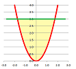
Example. Evaluate this area of the region is bounded by the parabola $y=x^2$ and the horizontal line $y=3$. We will need some algebra this time, to find $a,b$:
The intersection points $(x,y)$ satisfy: $y=3=x^2$. Then $a=-\sqrt{3},\ b=\sqrt{3}$. We also realize from the sketch that $f(x)=3$ and $g(x)=x^2$. Then, $$\begin{array}{lll} \text{Area }&=\int_a^b(f-g)\, dx\\ &=\int_{-\sqrt{3}}^{\sqrt{3}}\left( 3-x^2 \right)\, dx\\ &=3x-\frac{1}{3}x^3\Bigg|_{-\sqrt{3}}^{\sqrt{3}}\\ &=\left( 3\sqrt{3}-\frac{1}{3}\sqrt{3}^3\right) - \left( -3\sqrt{3}-\frac{1}{3}(-\sqrt{3})^3\right)\\ &=2\left( 3\sqrt{3}-\frac{1}{3}\sqrt{3}^3\right)\\ &=2\left( 3\sqrt{3}-\sqrt{3}\right)\\ &=4\sqrt{3}. \end{array}$$ $\square$
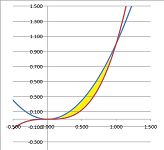
Example. Evaluate the area between $y=x^2$ and $y=x^3$. Once again, we find the intersection points by solving $x^2=x^3$. We have $a=0$ and $b=1$, which confirms the sketch and the fact that $x^3<x^2$:
Then, $$\begin{array}{lll} \text{Area }&=\int_a^b(f-g)\, dx\\ &=\int_{0}^{1}\left( x^2-x^3 \right)\, dx\\ &=\frac{1}{3}x^3-\frac{1}{4}x^4\Bigg|_{0}^{1}\\ &=\frac{1}{3}-\frac{1}{4}\\ &=\frac{1}{12}. \end{array}$$ $\square$
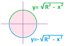
Example (circle). Let's revisit the computation of the area of the circle:
This time we don't have to split it in half and rely on its symmetry; the circle is the region between two graphs: $$y=\sqrt{R^2-x^2} \text{ and } y=-\sqrt{R^2-x^2}.$$ The former is $f$ and the letter is $g$. Also, $a=-R,\ b=R$. Then, $$\text{Area }=\int _{-R}^R\left(\sqrt{R^2-x^2} +\sqrt{R^2-x^2} \right)\,dx=2\int _{-R}^R\sqrt{R^2-x^2}\,dx = \pi R^2.$$ The integral is evaluated via a trig substitution, just as before. $\square$
Exercise. Find the area of the intersection of the two regions bounded by the circles $x^2+y^2=1$ and $(x-1)^2+y^2=1$.
Exercise. Find the area between the curves $x=y^2$ and $x=y^4$. Hint: transform the plane first.
Riemann integrals are like areas but, unlike areas, they may be positive or negative. The area “under” can be positive or negative, but the area “between” should always positive.
The linear density and the mass
The method that starts to shape up is the following. Suppose we have a quantity $Q$ “contained” in a space region $R$: area, volume, mass (below), etc. Then,
- we represent the total quantity $Q$ as the sum of its values $Q_i$ over simpler, or smaller, regions of $R$;
- we represent, or approximate, each of these values via a familiar quantity, e.g., area via length, volume via area etc.;
- we recognize the sum as the Riemann sum of a function that represents some other quantity $q$ spread over the region; and finally
- the quantity $Q$ is equal to the integral of $q$.
The last step is necessary only when we approximate an idealized situation.
Let's illustrate the method with one more example.
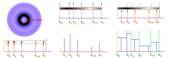
Recall how the linear density was defined. We are given a metal rod:
The rod might be non-uniform, i.e., the density varies but only in the horizontal direction. For example, this might happen when two metals are (imperfectly) melted into a piece of alloy:
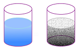
Another example is particles suspended in a liquid that settles -- because of gravity -- in a pattern that is denser at the bottom:
In either case, there is a line (we call it the $x$-axis) with no change in density in the directions perpendicular to it. We then ignore those directions and the density becomes a function of a single number $x$ designating the location along this line; hence the linear density $y=l(x)$.
Take a small piece of the rod at location $x$, $\Delta x$ long, and let's call its mass $\Delta m$. Then, for this piece, we have: $$\text{linear density} = \frac{\text{mass}}{\text{length}} = \frac{\Delta m}{\Delta x} = \frac{m(x + \Delta x) - m(x)}{\Delta x}.$$
Let's reverse this analysis. Suppose this time the linear density $l$ is given, what is the mass of the rod?
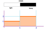
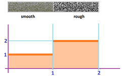
Example (two pieces). Suppose the two metals haven't merged at all:
Therefore, the mass is simply the sum of the two: $1\cdot 1+2\cdot 1= 3$. It is also the area of the two rectangles under the graph of the density function $l$, which is a step-function, and, therefore, the integral of $l$ over $[0,2]$. $\square$
Exercise. What if the two rods have lengths $.5$ and $1.5$?
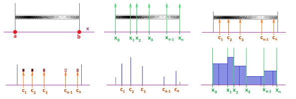
Instead of just pointing out what $m$ is, let's start from scratch. We have an augmented partition $P$: $$a=x_0\le c_1\le x_1\le ... \le c_n\le x_n=b,$$ with these lengths of segments: $$\Delta x_i=x_i-x_{i-1}.$$
We first imagine that the rod is divided into smaller pieces so that the density of each is found separately: $F_1,F_2,...,F_n$. Then the total weight is simply $$\text{total weight }= F_1\Delta x_1+F_2\Delta x_2+...+F_n \Delta x_n.$$ The formula is sufficient for applications when an approximation is sufficient.
Here, we assume that the density is changing continuously and we cut the rod into these small segments by the planes starting at $x=x_i$ and then sample its density at the points $c_i$:
Then the density of each segment -- if uniform -- is given by $l(c_i)$ and we have: $$\text{mass of }i\text{th segment}= \text{density}\cdot \text{length}=l(c_i)\cdot \Delta x_i.$$ Then, $$\text{total mass }= \sum_{i=1}^n l(c_i)\cdot \Delta x_i.$$ We recognize this expression as the Riemann sum, $\sum_{[a,b]} l\, \Delta x $, of the linear density function over this partition.
Definition. If a function $l$ defined at the secondary nodes of a partition of a segment $[a,b]$ is called a linear density then its Riemann sum $\sum_{[a,b]} l\, \Delta x $ is called the mass of the segment.
Now, what if the density varies continuously?
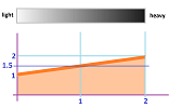
Example (linear dependence). Suppose the density of a rod of length $2$ is changing linearly: from $1$ to $2$. Then the meaning of the average density is clear; it is $1.5$.
Therefore, the mass is $1.5\cdot 2= 3$. It is also the area of the triangle under the graph of the density function $l(x)=1+x/2$ and, therefore, the integral of this function over $[0,2]$. $\square$
If the density is variable, then the mass of each segment -- when short enough -- is approximated by the mass of such a segment made entirely of material of density $l(c_i)$: $$\text{mass of }i\text{th segment}\approx \text{density}\cdot \text{length}=l(c_i)\cdot \Delta x_i,$$ and $$\text{total mass }\approx \sum_{i=1}^n l(c_i)\cdot \Delta x_i =\sum_{[a,b]} l\, \Delta x.$$ Then, we define the mass of the rod as the limit, if it exists, of these Riemann sums, i.e., the Riemann integral of $l$: $$\text{mass }=\int_a^bl\, dx.$$
Definition. If an integrable function $l$ on segment $[a,b]$ is called a linear density then its Riemann integral $\int_a^bl\, dx$ is called the mass of the segment.
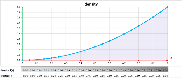
Example (quadratic dependence). Suppose we have again a rod of length $2$ with the density changing from $1$ to $2$, but quadratically, $l(x)=x^2+1$. The mass is impossible to guess:
Then, $$\text{mass }=\int_a^b l\, dx=\int_0^1 (x^2+1)\, dx=\frac{x^3}{3}+x\bigg|_0^1=\frac{4}{3}.$$ $\square$
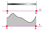
Here is another way to explain our definition. We realize that every location with higher density simply contains more material and we can just spread it out -- vertically -- making a plate that is wider at this spot and thinner at the location with a lower density:
In reverse, imagine that the area under the graph is made of a sheet of metal and the is rolled into a non-uniform rod.
Exercise. Find how the mass of a rod with an exponentially growing density grows.
The Fundamental Theorem of Calculus provides further insight. Suppose $m(x)$ is the weight of the rod from $a$ to $x$. Then the derivative of this function is the density: $$m'(x)=l(x).$$
Exercise. Is meaningful to speak of the mass of an infinitely long rod?
The center of mass
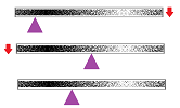
Can we now balance this non-uniform rod on a single point of support?
The question is important because this point, called the center of mass, is the center of rotation of the object when subjected to a force.
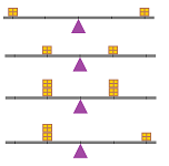
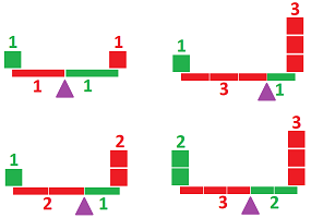
The analysis starts with a simplest case, seesaw. Two persons of equal weight will be in balance when located at equal distance from the point of support.
Now, what can be changed? What if one person is heavier than the other? From experience, we know that the latter person should sit farther from the center in order to balance the beam. In fact, the distance should be twice as long!
Conversely, if one person sits farther from the center than the other of the same weight, the former person should be joined by another in order to balance the beam.
Suppose the shorter distance is $a$ and the smaller weight is $m$. Then, combined, the distances are $a$ and $2a$ and weights are $2m$ and $m$. We express this data via the balance equation: $$(a)(2m)=(2a)(m).$$
In other words, this expression: $$\text{ distance }\cdot \text{ weight },$$ called the moment, is the same to the left and to the right of the support. This distance is also called the lever.
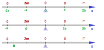
Let's add the $x$-axis.
We then realize that it is the signed distance, i.e., the $x$-coordinate, of the object that matters. We simply re-write the balance equation: $$(-a)(2m)+(2a)(m)=0.$$
Then, $$\text{ moment }= \text{ coordinate }\cdot \text{ weight }.$$ Furthermore, we can assume there is an object at every location but the rest of them have $0$ mass. The balance equation becomes: $$...+(-2a)(0)+(-a)(2m)+(0)(0)+(a)(0)+(2a)(m)+...=0.$$
This analysis brings us to the idea of combining the weights and the distances in a proportional manner in order to evaluate the contribution of a particular weight to the overall balance. The balance equation simply says that the sum of all moments is $0$.
Definition. We call a system of weights any collection of non-negative numbers $m_1,...,m_n$ called weights assigned to $n$ locations with coordinates $a_1,...,a_n$ on the $x$-axis.
Definition. The total moment of the system of weights with respect to the origin is defined to be the sum of the moments of the weights, i.e., $$\sum_i m_i a_i.$$ The balance equation of the system states that its total moment is zero.
Example. With this insight, let's confirm that an object is balanced.
$\square$
We now go back to the original problem. Suppose different weights are located on a beam, where do we put the support in order to balance it?
It was entirely our decision to place the origin of our $x$-axis at the center of mass. The result we have established should be independent from that choice and we can move the origin anywhere.
We just need to execute a change of variables. Suppose the center of mass (and the origin of the old coordinate system) is located at the point with coordinate $c$ of the new coordinate system. Then, the new coordinate of the $i$th object is $$c_i=a_i+c.$$ Therefore, the balance equation has this form: $$\sum_i m_i (c_i-c)=0.$$
Alternatively, we have: $$\sum_i m_i c_i=c\sum_i m_i.$$ It's as if the whole weight is concentrated at $c$. Hence the name.
Definition. Suppose we have a system of weights $m_1,...,m_n$ located at $c_1,...,c_n$ on the $x$-axis. For a given point $c$ and for each $i$, the product $$m_i(c_i-c)$$ is called the $i$th weight's moment with respect to $c$. The sum of the moments, $$\sum_i m_i (c_i-c),$$ is called the total moment with respect to $c$. The center of mass of this system of weights is such a point $c$ that the total moment with respect to $c$ is zero.
Of course, if $c=0$, we have the old definition.
Example. Following this insight, let's find the center of mass of an object. The method amounts to trial and error. We just move $c$ while watching the total moment.
$\square$
Exercise. What if we allow the values of $m_i$ to be negative? What is the meaning of the system and of $c$?
To make our task easier, we solve the balance equation for $c$.
Theorem. If $c$ is the coordinate of the center of mass of the system of weights, then $$c=\frac{\sum_i m_i c_i}{\sum_i m_i}.$$
Exercise. Prove the formula.
In other words, $$\text{center of mass }=\frac{\text{total moment}}{\text{total mass}}.$$
Example. Armed with this formula, we can quickly find the centers of mass of many objects.
$\square$
Example. Let's test the formula for a system of just two objects. First, suppose we have two identical weights located at $a$ and $b$. Then $$c=\frac{ma+mb}{m+m}=\frac{a+b}{2}.$$ So, no matter what the weight is, the center of mass lies halfway between the two objects, as expected. What if the weights are different? We can guess that the center of mass will be closer to the heavier object. But by how much? Suppose these are $m$ and $2m$. We compute: $$c=\frac{ma+2mb}{m+2m}=\frac{a+2b}{3}=\frac{1}{3}a+\frac{2}{3}b.$$ It's twice as close to the heavier object (bottom left):
$\square$
In general, the proportion of the distance is the proportion of the weight.
Exercise. If $\alpha$ and $\beta$ are the shares of the total weight, where is the center of mass of this two-object system?
More generally, the coordinate of the center of mass of the system can be re-written: $$c=\frac{\sum_i m_i c_i}{\sum_i m_i}=\sum_i\frac{ m_i }{\sum_j m_j} c_i.$$ Therefore, we have the following.
Corollary. If $c$ is the coordinate of the center of mass of a system of weights with locations at $c_i$ and relative weights $\mu_i$, then $$c=\sum_i \mu_i c_i.$$
Notice that the numerous weights placed on the bar start to look like the graph of a function! The value of this function is the height of the blocks placed at that location. We know, however, that this function is also seen as the linear density of a rod.
Next, let's imagine that the density varies in a more unpredictable way.
We continue in the same way as in the last section -- an augmented partition $P$ of interval $[a,b]$ is given: $$a=x_0\le c_1\le x_1\le ... \le x_{n-1}\le c_n \le x_n=b.$$ Then the density function $l$ is defined at the secondary nodes. Then the terms $l(c_i)\Delta x_i$ representing the weight of each interval are formed... but not added this time.
Each of these terms is a weight placed on top of the interval visualized as a rectangle. However, it is assumed that the weight of the $i$th rectangle is concentrated at $c_i$. The lever of each weight is also shown. Then the total moment of this system of weights with respect to some $c$ is the following: $$\sum_i m_i (c_i-c)=\sum_i l(c_i)\, \Delta x_i (c_i-c)=\sum_i l(c_i) (c_i-c)\, \Delta x_i.$$ Have we produced a Riemann sum as before? Well, this isn't the Riemann sum of $l$! Let's try this function (dependent on our choice of $c$): $$f(x)=l(x)(x-c).$$ Then, indeed, we face its Riemann sum: $$\sum_i m_i (c_i-c)=\sum_{[a,b]} f\, \Delta x.$$ Just as above, the system of weights that makes up the rod is balanced when the total moment is zero: $$\sum_{[a,b]} l(x)(x-c)\, \Delta x=0.$$ We arrive to a similar conclusion below.
Theorem. Suppose a function $y=l(x)$ is defined at the secondary nodes $c_i,\ i=1,2,...,n$, of a partition of interval $[a,b]$. Then the system of weights $l(c_i)\Delta x_i,\ i=1,2,...,n$, has its center of mass at the following point: $$c=\frac{\sum_{[a,b]} l(x)x\, \Delta x }{\sum_{[a,b]} l(x) \, \Delta x }.$$
What we have discovered is that the problem of balancing a rod with a variable density is equivalent to the problem of balancing the region below the graph of the density function:
Example. Let's test this formula on some regions cut from the unit circle:
In Chapter 14, we will offer more complex examples. $\square$
Exercise. Prove that if the density of the rod is strictly increasing (or decreasing), its center of mass cannot be in the center.
The next step is to think of the weights assigned to every location on the $x$-axis. In other words, the distribution of weight is no longer incremental.
What we have learned is that the total moment of the region with respect to some $c$ is approximated by that of this system of weights, which is the Riemann sum, $$\sum_i m_i (c_i-c)=\sum_i l(c_i)\, \Delta x_i (c_i-c)=\sum_{[a,b]} f\, \Delta x,$$ of the function $$f(x)=l(x)(x-c).$$ The beam doesn't have to be balanced and the total moment doesn't have to be zero for each partition, but it does have to diminish to zero as we refine the partition. This means that the Riemann integral of this function is zero.
Definition. Suppose we have a non-negative function $y=l(x)$ integrable on segment $[a,b]$ called the density function. For a given point $c$, the integral $$\int_a^b l(x)(x-c)\, dx$$ is called the total moment of the segment with respect to $c$. The center of mass of the segment with density function $l$ is such a point $c$ that the total moment with respect to $c$ is zero.
Theorem. Suppose we have a non-negative function $y=l(x)$ integrable on interval $[a,b]$. If the mass of the segment is not zero, then the center of mass is: $$c=\frac{\int_a^b l(x)x\, dx}{\int_a^b l(x)\, dx}.$$
Proof. First, we note that $y=l(x)(x-c)$ is integrable by PR. Then we use SR and CMR to compute the following: $$0=\text{ total moment }=\int_a^b l(x)(x-c)\, dx=\int_a^b l(x)x\, dx+c\int_a^b l(x)\, dx.$$ Now solve for $c$. $\blacksquare$
Once again, $$\text{center of mass }=\frac{\text{total moment}}{\text{total mass}}.$$
Exercise. Show this theorem implies the previous one.
Example (linear dependence). Suppose the density of a rod of length $2$ is changing linearly: from $1$ to $2$, i.e., $l(x)=x/2+1$.
Then, the mass is $3$. It was found in the last section based on a common sense analysis. That's the denominator of the fraction. Now, the numerator. Just the common sense won't help this time; we need to integrate: $$\begin{array}{ll} \int_0^2 l(x)x\, dx&=\int_0^2 (x/2+1)x\, dx\\ &=\int_0^2 (x^2/2+x)\, dx\\ &=x^3/6+x^2/2\Bigg|_0^2\\ &=8/6+4/2\\ &=10/3. \end{array}$$ Therefore, the center of mass is $$c=\frac{10}{3}\div 3=\frac{10}{9}.$$ Slightly to the right of the center... $\square$
Exercise. Find the center of mass of a rod with a linearly increasing density.
Exercise. Find the center of mass of a plate cut from a circle of radius $1$ centered at the origin by the lines $x=a$ and $x=b$.
Exercise. What is the meaning of the center of mass of an infinite object?
The radial density and the mass
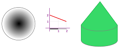
Suppose next we have an alloy that is rotated as it hardens. Then its density depends (only) on the distance from the center.
The same effect is produced by stirring a liquid.
In either case, we ignore the depth and all we see is a disk. Then, for any radial line (we pick one and call it the $x$-axis) there is no change in density in the directions perpendicular to it. We then ignore those directions and the density becomes a function of a single number $x$ designating the distance to the center along this line; hence the radial density $y=r(x)$.
We will provide analysis similar to the above to define the mass of such an object.
Suppose the radial density $r$ is given, what is the mass of the disk?
Example (two pieces). Suppose the two metals with densities $2$ on the inside and $1$ on the outside haven't merged at all. The object is simply a combination of a disk of radius $1$ and a washer around it of thickness $1$:
Then, the mass is simply the sum of the mass of the disk and the mass of the washer: $$\begin{array}{lll} \text{mass }&=2\cdot\text{area of the disk }&+ 1\cdot\text{area of the washer }\\ &=2\cdot \pi \cdot 1^2 &+1\cdot (\pi \cdot 2^2-\pi \cdot 1^2). \end{array}$$ It's $5\pi$. $\square$
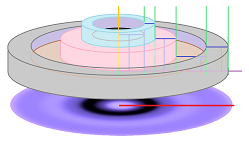
We can just replace the disk that has a constant thickness and a variable density with one that has a variable thickness and a constant density. Then we can use the results of the last section. Instead we start from scratch.
Suppose we have an augmented partition $P$ of the radius: $$a=x_0\le c_1\le x_1\le ... \le c_n\le x_n=b.$$ Here, we cut the disk into small washers by the cylinders starting at $x=x_i$ and then sample its density at the points $c_i$:
Then the density of each washer -- when uniform -- is $r(c_i)$ and we have: $$\text{mass of }i\text{th washer }= \text{density}\cdot \text{area}=r(c_i)\cdot\left( \pi x_i^2 -\pi x_{i-1}^2 \right),$$ since the inside radius of the washer is $x_{i-1}$ and the outside is $x_i$.
Then, $$\text{total mass }= \sum_{i=1}^n r(c_i)\cdot \pi\left( x_i^2 -x_{i-1}^2 \right).$$ This formula is fine for computations but it is not the Riemann sum of any function... A clever trick is to choose the secondary nodes to be the mid-points: $$c_i=\frac{1}{2}(x_i+x_{i-1}).$$ Then, we can factor the difference of two squares and simplify: $$\text{total mass }= \sum_{i=1}^n r(c_i)\cdot \pi( x_i +x_{i-1})( x_i -x_{i-1})= 2\pi \sum_{i=1}^n r(c_i)c_i\cdot \Delta x_i.$$ This is the Riemann sum of a simple function. Then, we define the mass of the disk as: $$\text{mass }=2\pi \sum_{[a,b]} xr(x) \, \Delta x.$$
What if the density varies continuously?
Then the mass of each washer -- when thin enough -- is approximated by the mass of such a washer made entirely of material of density $r(c_i)$: $$\text{mass of }i\text{th washer }\approx \text{density}\cdot \text{area}=r(c_i)\cdot\left( \pi x_i^2 -\pi x_{i-1}^2 \right).$$ Then we go through the same algebra: $$\text{total mass }\approx \sum_{i=1}^n r(c_i)\cdot \pi\left( x_i^2 -x_{i-1}^2 \right)= 2\pi \sum_{i=1}^n r(c_i)c_i\cdot \Delta x_i.$$ Then, we define the mass of the disk as the limit of these Riemann sums; i.e., $$\text{mass }=2\pi\int_a^b xr(x)\, dx.$$
Definition. If an integrable function $r$ on segment $[0,b]$ is called a radial density then the above integral is called the mass of the disk of radius $b$.
Once again, we realize that each location with higher density simply contains more material and we can just spread it out -- vertically -- making the disk thicker at this spot and thinner at the location of lower density.
Example (linear dependence). Suppose the density of a disk of radius $2$ is changing linearly: from $1$ to $2$. Then the meaning of the average density depends on the respective areas, as shown above.
The mass must have something to do with the volume of this surface of revolution... Let's integrate: $$\begin{array}{lll} \text{mass }&=2\pi\int_a^b xr(x)\, dx\\ &=\pi\int_0^2 x(2-x/2)\, dx\\ &=\pi\int_0^2 (2x-x^2/2)\, dx\\ &=\pi(x^2-x^3/6)\bigg|_0^2\\ &=\pi(2^2-2^3/6)\\ &=\frac{8\pi}{3}. \end{array}$$ $\square$
The flow velocity and the flux
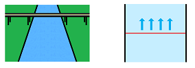
Suppose water flows in a canal:
How much water is crossing the given line per unit of time? We will ignore the depth.
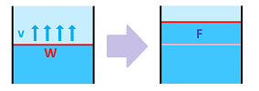
When the velocity of the water is the same at all locations, the total amount of the water that has crossed the line, called the flux $F$, is the velocity $v$ times the width $W$ of the cross-section: $$F=v\cdot W.$$
The flow velocity may vary depending on the location (not time!). We assume that the velocity is the same along the lines parallel to the walls of the canal. We visualize the process by imagining that a narrow strip of red dye is applied across the canal and then after, say, one minute we see how the die has progressed:
What is the flux then?
To begin with, we assume that the flow velocity depends on a single variable (one degree of freedom again), the location distance across the canal. Then, there is a line -- we choose it to be interval $[a,b]$ on the $x$-axis -- with no change in velocity in the directions perpendicular to it. Then the velocity is a function $y=v(x)$ of a single number $x$ in $[a,b]$.
Suppose this time the velocity $v$ is given as a function of location, what is the flux?
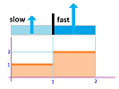
Example (two gates). Suppose we have two separate canals side by side, with the velocities $1$ and $2$ and the same width $1$:
Therefore, the volume is simply the sum of the two: $1\cdot 1+2\cdot 1= 3$. It is also the area of the two rectangles under the graph of the velocity function $v$, which is a step-function, and, therefore, the integral of $l$ over $[0,2]$. $\square$
Instead of just pointing out that the flux is an antiderivative of the speed (with respect to location not time!), let's start from scratch. We have an augmented partition $P$: $$a=x_0\le c_1\le x_1\le ... \le c_n\le x_n=b.$$
We first imagine that the canal is divided into channels or locks so that the flow velocity through each is found separately: $F_1,F_2,...,F_n$. Then the total flow is simply $$\text{total volume }= F_1\Delta x_1+F_2\Delta x_2+...+F_n \Delta x_n.$$ The formula is sufficient for practical applications.
Next, we would like to find a Riemann sum here. We imagine that the flow velocity varies incrementally over the gates that divide the canal's cross-section. The canal is cut into segments by the line starting at $x=x_i$ and sampled velocity at the points $c_i$ is $v(c_i)$:
Then we have: $$\text{flux though }i\text{th segment}= \text{velocity}\cdot \text{width}=v(c_i)\cdot \Delta x_i.$$ Then, $$\text{total flux }= \sum_{i=1}^n v(c_i)\cdot \Delta x_i.$$ We recognize this expression as the Riemann sum, $\sum_{[a,b]} v\, \Delta x$, of the velocity function over this partition.
Definition. If a function $v$ defined at the secondary nodes of a partition of a segment $[a,b]$ is called a flow velocity then its Riemann sum $\sum_{[a,b]} v \, \Delta x $ is called the flux: $$\text{flux }=\sum_{[a,b]} v \, \Delta x.$$
What if the flow velocity varies continuously?
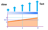
Example (linear dependence). Suppose the velocity of the canal of width $2$ is changing linearly: from $1$ to $2$. Then the meaning of the average velocity is clear; it is $1.5$.
Therefore, the volume is $1.5\cdot 1= 1.5$. It is also the area of the triangle under the graph of the velocity function $v(x)=1+x$ and, therefore, the integral of $v$ over $[0,2]$. $\square$
Then the flux through each segment -- when short enough -- is approximated by the volume with the water moving entirely at the velocity $v(c_i)$: $$\text{volume of }i\text{th segment}\approx \text{velocity}\cdot \text{width}=v(c_i)\cdot \Delta x_i.$$ Then, $$\text{total volume }\approx \sum_{i=1}^n v(c_i)\cdot \Delta x_i.$$ We define the volume of the rod as the limit, if it exists, of these Riemann sums, i.e., the Riemann integral of $v$: $$\text{flux }=\int_a^bv\, dx.$$
Definition. If an integrable function $v$ on segment $[a,b]$ is called a flow velocity in a canal then its Riemann integral $\int_a^b v\, dx$ is called the flux.
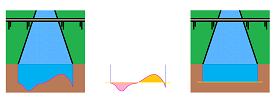
Here is another way to explain this result. We can take our canal, with a variable water velocity, and imagine a canal with the same flux but a constant velocity. How is it possible? We think of each location with higher velocity as one that has more water.
The first approach is to spread the water out -- vertically -- making the canal deeper at this spot and shallower at the location with a lower velocity:
The second approach is to think of each location with higher velocity as simply one with denser liquid.
Exercise. What if this is an ocean, i.e., the cross-section of our “canal” is infinitely wide?
A variation of this analysis is as follows. Suppose now that the water flows through a pipe:
Suppose the flow velocity varies depending on the distance from the location to the pipe's wall. For example, the water may go slower next to the wall because of the friction. We have a circular pattern again...
Definition. If an integrable function $v$ on segment $[0,R]$ is called a flow velocity through a pipe of radius $R$ then the Riemann integral $2\pi\int_0^R xv(x)\, dx$ is called the flux.
Exercise. Following the ideas developed in this chapter, justify the above definition.
The force and the work
Suppose a ball is dropped on the ground from a certain height:
This phenomenon is the result of the gravitational force. This force is directed down, just as the movement of the ball. The work done on the ball by this force as it falls is equal to the (signed) magnitude of the force, i.e., the weight of the ball, multiplied by the (signed) distance to the ground, i.e., the displacement. All horizontal motion is ignored as unrelated to the gravity.
The need for using the signed distance $D$ and force $F$ is revealed by the example of moving an object up from the ground. Then the work $W$ performed by the gravitational force is negative!
Of course, the sign in either case is determined by the direction of the axis we assign to the line of motion.
Suppose we are to move from point $a$ on the $x$-axis to point $b>a$. When the force $F$ is constant, the work $W$ is equal to the force $F$ times the distance covered between $a$ and $b$: $$W=F\cdot (b-a).$$
The force may vary depending on the location between $a$ and $b$.
Example (physics). The examples we have seen previously are: spring, gravitation, air pressure.
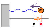
In the case of an object attached to a spring, the force is proportional to the (signed) distance of the object to its equilibrium according to the Hooke's Law: $$F(x)=-kx.$$
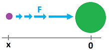
Away from the ground, the gravity is proportional to the reciprocal of the square of the distance of the object to the center of the planet according to the Newton's Law of Gravitation: $$F(x)=-\frac{k}{x^2}.$$ The pressure and, therefore, the medium's resistance to motion may change arbitrarily. $\square$
Example (traction). Suppose the force is traction and there are two distinct strips: one is smoother and the other rougher.
The force takes -- between $a=0$ and $b=2$ -- only two different values $1$ and $2$ switching at $c=1$. Therefore, the work is simply the sum of the two over either of the segments: $1\cdot 1+2\cdot 1= 3$. It is also the area of the two rectangles under the graph of the force function $F$, which is a step-function, and, therefore, the integral of $l$ over $[0,2]$. $\square$
We have an augmented partition $P$: $$a=x_0\le c_1\le x_1\le ... \le c_n\le x_n=b.$$ The path is divided into small segments by $x=x_i$ and then the force is sampled at the points $c_i$. Then the force on each segment -- if constant -- is equal to $F(c_i)$ and we have: $$\text{ work on }i\text{th segment}= \text{ force }\cdot \text{ length}=F(c_i)\cdot \Delta x_i.$$ Then, $$\text{total work }= \sum_{i=1}^n F(c_i)\cdot \Delta x_i.$$ Once again, we recognize this expression as the Riemann sum, $\sum_{[a,b]} F\, \Delta x $, of the force function over this partition. Then, we define the work of the force as this Riemann sums: $$\text{ work }=\sum_{[a,b]} F\, \Delta x.$$
Definition. If a function $F$ is defined at the secondary nodes of a partition of a segment $[a,b]$ is called a force function then its Riemann sum $\sum_{[a,b]} F \, \Delta x $ is called the work of the force over interval $[a,b]$.
What if the force varies “continuously”?
Example (linear dependence). Suppose the force is changing linearly over the interval $[0,2]$: from $1$ to $2$. Then the meaning of the average force is clear; it is $1.5$.
Therefore, the work is $1.5\cdot 2= 3$. It is also the area of the triangle under the graph of the force function $F(x)=1+x/2$ and, therefore, the integral of this function over $[0,2]$. When the change of the force is non-linear, the argument fails. $\square$
The work on each segment is approximated by the work with the force being constantly equal to $F(c_i)$: $$\text{ work on }i\text{th segment}\approx \text{ force }\cdot \text{ length}=F(c_i)\cdot \Delta x_i.$$ Then, $$\text{total work }\approx \sum_{i=1}^n F(c_i)\cdot \Delta x_i.$$ We define the work of the force as the limit, if it exists, of these Riemann sums, i.e., the Riemann integral of $F$: $$\text{ work }=\int_a^b F\, dx.$$
Definition. If an integrable function $F$ on segment $[a,b]$ is called a force function then its Riemann integral $\int_a^b F\, dx$ is called the work of the force over interval $[a,b]$.
Exercise. How much work does it take to move an object attached to a spring $s$ units from the equilibrium?
Exercise. How much work does it take to move an object $s$ units from the center of a planet?
As a summary, we have solved the problem of finding a certain quantity $W$ -- work, flow, and mass -- in an identical manner. We have an augmented partition $P$: $$a=x_0\le c_1\le x_1\le ... \le c_n\le x_n=b.$$
We divide the path into small segments by $x=x_i$ and then sample quantity $F$ -- the force, or the flow speed, or the linear density -- at the points $c_i$. Then this quantity, $F(c_i)$, on each segment is used to find the value of $W$: $$W_i= \text{ force }\cdot \text{ length}=F(c_i)\cdot \Delta x_i.$$
Then, the total approximated value of $W$ over the whole segment is $$\sum_i W_i= \sum_{i=1}^n F(c_i)\cdot \Delta x_i,$$ which is the Riemann sum of $F$ over this partition. The exact value of the total of $W$ is the limit of these Riemann sums, i.e., the Riemann interval of $F$: $$W=\int_a^b F\, dx.$$
Warning: in spite the common approach presented here, the treatments of the three integrals are substantially different in dimension $3$ (Chapters 20 and 21):
- the work is an integral over a curve;
- the flow is an integral over a surface;
- the mass is an integral over a solid.
We now consider a different setup...
We arrived at the integral formula above because of a simple (“additive”) property of work:
- when there are two segments of the trip, the work to move through the two is equal to the work required to move through the first plus the work required to move through the second.
We are to consider a situation when
- two objects, possibly identical, under a force, possibly constant, have to be moved different distances.
Then there is no such a shortcut formula.
Example (bricks). An example of such a task is stacking bricks:
Then the work -- of the person acting against the gravity -- is $$W=M\cdot 0\cdot h+M\cdot 1\cdot h+M\cdot 2 \cdot h+M\cdot 3\cdot h,$$ where $M$ is the weight of the brick and $h$ is its height. $\square$
Generally, what if the force is constant but the object isn't thought of as a point anymore. In other words, different parts of the object will travel different distances. This situation isn't covered by the above definition of work.
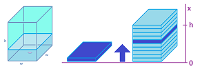
Example (cubical tank). Suppose we are to fill a tank with $w\times w$ base and height $h$ with water -- from the bottom:
What is the work required assuming that the density is $1$?
We imagine that water appears at the bottom in thin slices and then each is delivered to the appropriate height. They come from an augmented partition $P$ of $[0,h]$. This means that the $x$-axis is vertical. The $i$th slice is a square between the planes $x=x_{i-1}$ and $x=x_i$. Its thickness is $\Delta x_i=x_i-x_{i-1}$ and its weight is $w^2\cdot \Delta x_i$. Now, the $i$th slice is delivered to height $c_i$. The work to do so is $$w^2 \Delta x_i \cdot c_i.$$ Then the total work is approximated by: $$\text{work }\approx\sum_{i=1}^n w^2 c_i \cdot \Delta x_i.$$ This is the Riemann sum of the integral: $$\text{work }=w^2\int_0^h x\, dx=w^2\frac{h^2}{2}.$$ The result matches the idea that the work required is the same as the work to move the whole amount of water, volume $w^2h$, from the bottom to the average height within the tank, $h/2$. $\square$
Exercise. Suppose we are to fill a cylindrical tank with base of radius $R$ and height $h$ with water from the bottom. What is the work required?
Exercise. What if the horizontal cross-sections of the tank have arbitrary (but identical) shape?
Exercise. Suppose a chain of weight $M$ and length $h$ is to be pulled all the way up from the ground? What is the work required?
In the examples above, the work is repetitive. What if the cross section varies in shape and size?
Example (spherical tank). Suppose we are to fill a spherical tank of radius $R$ with water from the bottom:
What is the work required?
We imagine that water appears at the bottom in thin slices and then each is delivered to the appropriate height. They come from an augmented partition $P$ of $[-R,R]$. The $i$th slice is a disk between the planes $x=x_{i-1}$ and $x=x_i$. Its thickness is $\Delta x_i=x_i-x_{i-1}$, radius $r_i$ (to be found), and its weight is $\pi r_i^2\cdot \Delta x_i$. Now, the $i$th slice is delivered to location $c_i$ (depicted negative), covering the interval $[-R,c_i]$. The displacement is, therefore, $R+c_i$ and the work to do so is $$\pi r_i^2 \Delta x_i \cdot (R+c_i).$$ Then the total work is approximated by: $$\text{work }\approx\sum_{i=1}^n \pi r_i^2 (R+c_i) \cdot \Delta x_i.$$ Let's find the radius of the slice. From the Pythagorean Theorem, we have: $$r_i^2=R^2-c_i^2.$$ Then the above expression is the Riemann sum of the integral: $$\begin{array}{lll} \text{work }&=\pi\int_{-R}^R (R^2-x^2)(R+x)\, dx\\ &=\pi\int_{-R}^R \left( R^3-x^2R+R^2x-x^3 \right)\, dx\\ &=\pi \left( R^3x-\frac{1}{3}x^3R+R^2\frac{1}{2}x^2-\frac{1}{4}x^4 \right)\Bigg|_{-R}^R\\ &=\pi \left( R^4-\frac{1}{3}R^4+R^4\frac{1}{2}-\frac{1}{4}R^4 \right)-\pi \left( -R^4+\frac{1}{3}R^4+R^4\frac{1}{2}-\frac{1}{4}R^4 \right)\\ &=\frac{4}{3}\pi R^4. \end{array}$$ The result matches the idea that the work required is the same as the work to move the whole ball of water, volume $\frac{4}{3}\pi R^3$, so that its center of mass moves from $-R$ to $0$. $\square$
Exercise. Suppose we are to fill a “paraboloid” tank acquired by rotating the graph of $y=x^2$ around the $x$-axis, which is vertical, from the bottom. What is the work required?
Exercise. What work is needed to pull all the way up a chain hanging down if it is $10$ feet long and $20$ pounds heavy?
Exercise. What is the meaning of the work required over an infinite long trip?
The total and the average value of a function
What do these examples have in common?
A certain quantity, $f$, is “spread” around locations in space; for now, it is an interval within the $x$-axis. This quantity may be: length, area, density, velocity, force. When the quantity is (or is approximated by) a constant value within a segment of the interval, multiplying it by the length of this piece, $\Delta x$, gives us a new but still familiar quantity: $$\begin{array}{lll} \text{quantity } f& f\cdot \Delta x& \sum f\cdot \Delta x\\ \hline \text{length }& \text{ area }& \text{ total area }\\ \text{linear density }& \text{ mass }&\text{ total mass } \\ \text{flow rate }& \text{ flux }& \text{ total flux }\\ \text{force }& \text{ work }& \text{ total work }\\ \end{array}$$ When the quantity $f$ varies from segment to segment over the interval, it is represented by a function. When this change is incremental, the total value of $f$ is the sum of the terms $f\cdot \Delta x$, i.e., the Riemann sum of the function $f$. When this change is continuous, the total value of $f$ is approximated by this Riemann sum and, at the limit, it is the integral of $f$ over $[a,b]$.
Recall that the mean (or the average) of a quantity given by $n$ numbers $y_1,...,y_n$ is defined to be $$\text{mean }=\frac{y_1+y_2+...+y_n}{n}.$$ How should be understand the mean of a quantity that is continuously spread over a line segment, say $[a,b]$? The numerator would have infinitely many terms!
Let's start with the idea of a weighted average. We assume that we have $n$ weights, i.e., $n$ positive numbers $m_1,...,m_n$ with $$m_1+...+m_n=1.$$ Then for any given $n$ numbers $y_1,...,y_n$, we define their weighted average as follows: $$\text{weighted average }=m_1y_1+m_2y_2+...+m_ny_n=\sum_{i=1}^n m_i y_i.$$
Exercise. Show that the mean is the weighted average with $m_i=1/n$ for all $i$.
Example (scores). The weighted average may appear when one computes the total score in a class after several assignments of different weights. For example, this may be the grade breakdown:
- participation: $20\%$,
- quizzes: $30\%$,
- midterm: $20\%$,
- final exam: $30\% $.
Then the total score is the following weighted average of the five scores: $$\text{TOTAL }= .20 \times P + .30\times Q + .20\times M + .30\times F.$$ $\square$
Example. Recall that If $c$ is the coordinate of the center of mass of a system of weights with locations at $y_i$ and relative weights $m_i$, then $$c=\sum_i m_i y_i.$$ Therefore, the weighted average is the same, in this case, as the center of mass of the system. $\square$
If a substance is uniformly distributed over a segment of the line, the weight of the segment is proportional to its width. We are, then, justified to use these widths as substitutes for the weights in the weighted average. This is the main idea:
- each weight $m_i$ is the relative length of the interval where $y_i$ of the quantity is located.
We start with an augmented partition $P$ of the interval: $$a=x_0\le c_1\le x_1\le ... \le c_n\le x_n=b,$$ then $$m_i=\frac{\Delta x_i}{b-a}.$$ Let's substitute: $$\text{weighted average }=\sum_{i=1}^n\frac{\Delta x_i}{b-a}y_i=\frac{1}{b-a}\sum_{i=1}^n y_i\, \Delta x_i.$$ Furthermore, if these numbers are given by a function defined at the secondary nodes of the partition, $$f(c_i)=y_i,$$ then we have: $$\text{weighted average }=\frac{1}{b-a}\sum_{i=1}^n f(c_i)\, \Delta x_i.$$
This sum is the Riemann sum of this function!
Definition. The average value of a function $f$ defined at the secondary nodes of a partition of an interval $[a,b]$ is denoted and defined as $$\bar{f}=\frac{1}{b-a}\sum_{[a,b]} f\, \Delta x.$$
It is, in other words, the total value of $f$ per unit of length.
Warning: the average mass of a system of weights is not the same as the average location of the weights.
Example.
$\square$
What if the function doesn't change incrementally but “continuously”?
Example (linear dependence). Suppose the function $f$ is linear, from $1$ to $2$ over the interval $[0,2]$. Then the meaning of the average value is clear; it is $1.5$.
Where does it comes from? The area of the triangle under the graph of $f$, i.e., $3$, which is the integral of $f$ over $[0,2]$, divided by its length, $2$. $\square$
Then we think of the fraction above as an approximation of the average. This analysis justifies the following definition.
Definition. The average value of an integrable function $f$ over interval $[a,b]$ is denoted and defined as $$\bar{f}=\frac{1}{b-a}\int_a^b f\,dx.$$
To illustrate, consider how one levels an uneven surface of sand:
The average depth is illustrated below:
Both canals have the same amount of water.
Thus, by averaging we mean replacing any function, $y=f(x)$, with a constant function, $y=\bar{f}$, chosen so that the two have the same integral: $$\bar{f}\cdot (b-a)=\int_a^b f\, dx.$$
Exercise. Prove the above statement.
Theorem. Over a given interval, we have: (a) the average of the sum is the sum of the averages: $$\overline{f+g}=\bar{f}+\bar{g};$$ and (b) the constant multiple of the average is the average of the constant multiple: $$\overline{cf}=c\bar{f}.$$
Exercise. Prove the theorem.
Exercise. What can you say about the average of (a) an odd function, (b) an even function, (c) a periodic function, over $[-r,r]$?
We can rewrite the table with which we started the section: $$\begin{array}{lll} \text{} f& \int_a^b f\, dx& \quad &\frac{1}{b-a}\int_a^b f\, dx&\\ \hline \text{length }& \text{ total area }&\quad & \text{ average length }&\\ \text{linear density }& \text{ total mass }& \quad &\text{ average linear density }\\ \text{flux }& \text{ total flux }& \quad &\text{ average flux }\\ \text{force }& \text{ total work }& \quad &\text{ average force }\\ \end{array}$$ All have been introduced in the chapter except for the first item that comes from Chapter 11.
Exercise. What is the meaning of the average of a function defined on an infinite interval?
Numerical integration
To apply the integral formulas presented in this chapter, we need to evaluate those integrals. This is an ideal outcome: $$\text{area }=\int_0^2 x^2\, dx=\frac{x^3}{3}\bigg|_0^1=\frac{1^3}{3}-\frac{0^3}{3}=\frac{1}{3}.$$ We have an exact number. However, such an outcome is an exception not a rule! Some integrals do not produce familiar functions so that we can just plug in the two values. Conversely, some of the functions have been defined as integrals only, such as: $$\int e^{x^2}\, dx.$$ There is no other formula!
What do we do? The answer is in the definition of the Riemann integral. It is defined via Riemann sums and these sums serve as its approximations. We will assume below that all functions are integrable, which means that any choice of the secondary nodes for the Riemann sums is equally valid.
Example. Let's review the ways we estimate this integral of $f(x)= x^{2}$ over $[0,1]$: $$\int_0^1 f\, dx.$$
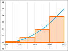
We choose the number of intervals to be $n=4$ with equal intervals of length $h=1/4$. Then we choose, as the secondary nodes, the left-end or the right-end of each interval:
At those points the function is evaluated. This is the computation of the left-end Riemann sum $L_4$: $$\begin{array}{r|cccccll} &\bullet&--&|&--&|&--&|&--&\bullet\\ x&0&&1/4&&1/2&&3/4&&1\\ x^2&0&&1/16&&1/4&&9/16&&1\\ L_4&0\cdot 1/4&+&1/16\cdot 1/4&+&1/4\cdot 1/4&+&9/16\cdot 1/4&& &\approx 0.22\\ \hline \sum_{[0,0]}&0\cdot 1/4&&&&&&&&&=0\\ \sum_{[0,1/4]}&0\cdot 1/4&+&1/16\cdot 1/4&&&&&&&\approx 0.04\\ \sum_{[0,1/2]}&0\cdot 1/4&+&1/16\cdot 1/4&+&1/4\cdot 1/4&&&&&\approx 0.10 \\ \sum_{[0,3/4]}&0\cdot 1/4&+&1/16\cdot 1/4&+&1/4\cdot 1/4&+&9/16\cdot 1/4&& &\approx 0.22 \end{array}$$ We, furthermore, realize that we are computing the Riemann sum function for this augmented partition. Its four values are shown in bottom of the table. $\square$
Warning: it is better to avoid “approximating with approximations” and replace the last number with its exact value: $$L_4=\frac{7}{32}=.21875.$$
Exercise. Create a table of values for the Riemann sum function for the right ends.
Example. We can also choose the mid-points as the secondary nodes:
This is the computation of the mid-point Riemann sum $M_4$ for the same integral: $$\begin{array}{r|ccccccll} &\bullet&--&|&--&|&--&|&--&\bullet\\ x&&1/8&&3/8&&5/8&&7/8&\\ f(x)=x^2&&(1/8)^2&&(3/8)^2&&(5/8)^2&&(7/8)^2&\\ M_4&&(1/8)^2\cdot 1/4&+&(3/8)^2\cdot 1/4&+&(5/8)^2\cdot 1/4&+&(7/8)^2\cdot 1/4&= 0.328125\\ \hline \sum_{[0,1/8]}&&(1/8)^2\cdot 1/4&&&&&&&\approx 0.004\\ \sum_{[0,3/8]}&&(1/8)^2\cdot 1/4&+&(3/8)^2\cdot 1/4&&&&&\approx 0.040\\ \sum_{[0,5/8]}&&(1/8)^2\cdot 1/4&+&(3/8)^2\cdot 1/4&+&(5/8)^2\cdot 1/4&&&\approx 0.230\\ \sum_{[0,7/8]}&&(1/8)^2\cdot 1/4&+&(3/8)^2\cdot 1/4&+&(5/8)^2\cdot 1/4&+&(7/8)^2\cdot 1/4&\approx 0.328\\ \end{array}$$ It is much closer than $L_4$ to the true value of the integral, $1/3$. $\square$
Exercise. We have previously used a spreadsheet to calculate the Riemann sum function for $L_n$. Create a spreadsheet to automate computations the Riemann sum function for $R_n$ and $M_n$.
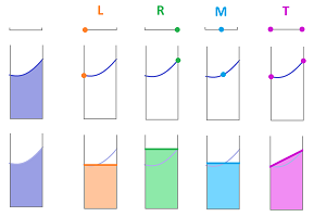
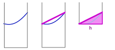
Thus, the Riemann sum chooses a point on the graph and then approximates its piece with a horizontal segment. The three choices are shown below.
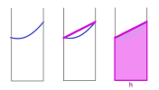
What if we choose two points -- at the end and the beginning of the interval -- and approximate this piece of the graph with a sloped line? It is, in fact, the familiar secant line! This third way to approximate the area is shown on far right.
Instead of a rectangle, we use a trapezoid. Its area is the average of the lengths of the two bases (vertical) multiplied by the height (horizontal):
Then the area of the trapezoid over the interval $[x_{k-1},x_k]$ is equal to $$\frac{f(x_{k-1})+f(x_k)}{2}h.$$ The sum of all $n$ of these is called the trapezoid approximation of the integral and denoted by $T_n$.
Exercise. Show that $T_n$ is the average of $L_n$ and $R_n$.
Example. Let's compute sum $T_4$ for the same integral. We use the same data and then add the following terms: $$f(x_{k-1})h+f(x_k)h$$ for each interval: $$\begin{array}{r|cccccll} &\bullet&--&|&--&|&--&|&--&\bullet\\ x&0&&1/4&&1/2&&3/4&&1\\ x^2&0&&1/16&&1/4&&9/16&&1\\ &0\cdot 1/4&+&1/16\cdot 1/4&&&&&& &\approx 0.016\\ &&&1/16\cdot 1/4&+&1/4\cdot 1/4&&&& &\approx 0.079\\ &&&&&1/4\cdot 1/4&+&9/16\cdot 1/4&& &\approx 0.203\\ &&&&&&&9/16\cdot 1/4&+&1\cdot 1/4 &\approx 0.391\\ \hline &&&&&&&&&\text{sum }&\approx 0.689\\ T_4&&&&&&&&&\text{half }&\approx 0.345\\ \end{array}$$ $\square$
Warning: the result is not a Riemann sum.
Exercise. Create a spreadsheet to automate computations of $T_n$.
These are the formulas for the four approximations: $$\begin{array}{ll} L_n=\sum_{i=1}^n f\big(a+(i-1)h\big)h;\\ R_n=\sum_{i=1}^n f\big(a+ih\big)h;\\ M_n=\sum_{i=1}^n f\big( a+(i-1)h+h/2 \big) h;\\ T_n=\sum_{i=1}^n\frac{1}{2}\bigg[ f\big(a+(i-1)h\big)+ f\big(a+ih\big) \bigg]h.\\ \end{array}$$
The expressions approximate the integral in the following sense.
Theorem. If $f$ is integrable on $[a,b]$ then, as $n\to \infty$, the sequences $L_n,\ R_n,\ M_n,\ T_n$ converge to $\int_a^b f\, dx$.
Only the last part needs proof.
Exercise. Prove the missing part. Hint: the Squeeze Theorem.
How well do these four perform?
- Question: For a given $n$, how close are we to the true value of the integral?
- Answer: we don't know, and we can't know, without some a priori knowledge.
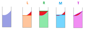
Since all four approximations are specific areas, the errors are also seen as certain areas:
Theorem. If $f$ is increasing on $[a,b]$, the left-end Riemann sum underestimates the integral while the right-end sum overestimates it: $$f\ \nearrow \ \Longrightarrow\ L_n\le\int_a^b f\, dx\le R_n;$$ meanwhile, when the function is decreasing the inequalities are reversed: $$f\ \searrow \ \Longrightarrow\ L_n\ge\int_a^b f\, dx\ge R_n.$$
In either case, the true value of the integral $I$ lies within between $R_n$ and $L_n$. In other words, the unknown $I$ must lie within a certain interval, either $$[L_n,R_n] \text{ or } [R_n,L_n] .$$
While the last result relies on monotonicity (and the derivative of $f$), for the other two approximations, a similar result relies on concavity (and the second derivative of $f$).
Theorem. If $f$ is concave down on $[a,b]$, the trapezoid sum underestimates the integral: $$f\ \frown \ \Longrightarrow\ T_n\le\int_a^b f\, dx;$$ meanwhile, when the function is concave up, the inequality is reversed: $$f\ \smile \ \Longrightarrow\ T_n\ge\int_a^b f\, dx.$$
We thus have discovered how these approximations err in different directions under different circumstances. However, the true measure of the quality of the approximation is the actual difference, i.e., the distance from the integral: $$\text{Error } = \bigg| \text{ Integral } - \text{ Approximation } \bigg|.$$ Since we don't know the value of the integral, we don't know the value of the error; we can only estimate it. This way we will know that we don't deviate from the truth too far.
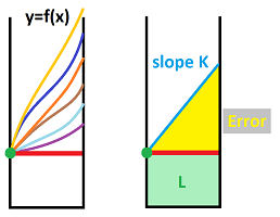
Let's take a look at the left-end approximation on a single interval. Suppose the only value that matters, $f(x_k)$, is known. Beyond that, we function can exhibit a variety of behaviors, including fast growth. The faster $f$ grows past $x_k$, the larger is the error of $L_n$. As the rate of this growth is limitless, so is our error (left):
Can we control the size of the error? Yes, if we are aware of -- a priori -- a limit on the rate of growth of $f$, i.e., its derivative. If the derivative is less than $K$, then the slope of the graph of $f$ is less than $K$ and, therefore, the graph will have to stay under the line with slope $K$ (right). This line is the worst-case scenario.
Note that such a restriction is expected to be possible when the derivative $f'$ is continuous according to the Boundedness Theorem (Chapter 6).
Theorem (Error estimate I). Suppose for all $x$ in $[a,b]$ we have $$|f'(x)|\le K_1,$$ for some real $K_1$. Then $$\left| L_n(f)-\int_a^b f\, dx \right|\le\frac{K_1(b-a)^2}{2n},$$ and $$\left| R_n(f)-\int_a^b f\, dx \right|\le\frac{K_1(b-a)^2}{2n}.$$
Proof. If we have an estimate for the derivative, $$f'(x)\le K,$$ on the whole domain of integration $[a,b]$, we have an estimate for the error on each interval first: $$\left| f(x_k)\Delta x-\int_{x_{k-1}}^{x_k} f\, dx \right|\le \frac{1}{2}(K \Delta x)\cdot \Delta x=\frac{1}{2}K \Delta x^2,$$ as the area of this triangle. Then we compute an estimate for the error of the left-end Riemann sum over the whole interval: $$\begin{array}{ll} E_n&=\left| L_n-\int_{a}^{b} f\, dx \right|\\ &=\left| \sum_{k=0}^{n-1} f(x_k)\Delta x-\sum_{k=0}^{n-1} \int_{x_{k-1}}^{x_k} f\, dx \right|\\ &=\left| \sum_{k=0}^{n-1} \left( f(x_k)\Delta x-\int_{x_{k-1}}^{x_k} f\, dx\right) \right|\\ &\le \sum_{k=0}^{n-1} \left| f(x_k)\Delta x-\int_{x_{k-1}}^{x_k} f\, dx \right|,&\text{ by the Triangle Inequality in Chapter 2}\\ &\le \sum_{k=0}^{n-1} \frac{1}{2}K \Delta x^2\\ &=\sum_{k=0}^{n-1} \frac{1}{2}K \left(\frac{b-a}{n}\right)^2\\ &=\sum_{k=0}^{n-1} \frac{1}{2}K \frac{(b-a)^2}{n^2}\\ &=\frac{1}{2}K \frac{(b-a)^2}{n}. \end{array}$$ $\blacksquare$
So, an a priori bound on the derivative gives an a priori bound on the error.
Example. Let's test this theorem on the integral $$\int_0^1 x^2\, dx=1/3,$$ with $L_4=0.22$ computed previously. First, we find the derivative: $$f(x)=x^2\ \Longrightarrow\ f'(x)=2x.$$ Then, we choose, of course, $$K_1=2.$$ Next, $$E_4=\frac{2(1-0)^2}{2 \cdot 4}=\frac{2}{8} = .25.$$ Then the integral's value should be within the interval: $$[L_4-E_4,L_4+E_4] = [.22-.25,.22+.25]=[-.03,.45].$$ A very crude but correct estimate! We can apply the theorem again, to the right-end approximation, resulting in an interval of the same size but centered around $R_4$: $$[R_4-E_4,R_4+E_4] = [.47-.25,.47+.25]=[.22,.72].$$ Furthermore, since the value $I$ of the integral belongs to both intervals, it belongs to their intersection: $$[-.03,.45] \cap [.22,.72]=[.22,.45].$$ Similarly, we have $I$ within $$[L_{10}-E_{10},L_{10}+E_{10}]=[.29-.1,.29+.1]=[.19,.39].$$ $\square$
Exercise. Find the interval for the above integral using $R_{10}$.
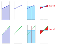
For contrast, let's take a look at the mid-point approximation. First suppose that $f$ is linear:
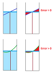
Even though the slopes are different, the error is the same, zero. It appears then that the derivative doesn't matter... Let's now add concavity:
The error isn't zero as in the former case. This observation suggests that the error is “created” by the second derivative of $f$.
Exercise. What difference does it make if $f$ concave down instead of up?
The idea of the last theorem was to use a bound for the derivative to make sure that the function doesn't deviate too far from its constant approximation (on each interval). Similarly, the idea of the next theorem is to use a bound for the second derivative to make sure that the function doesn't deviate too far from its linear approximation. We accept the result without proof.
Theorem (Error estimate II). Suppose for all $x$ in $[a,b]$, we have $$|f' '(x)|\le K_2,$$ for some real $K_2$. Then $$\left| M_n(f)-\int_a^b f\, dx \right|\le\frac{K_2(b-a)^3}{24n^2},$$ and $$\left| T_n(f)-\int_a^b f\, dx \right|\le\frac{K_2(b-a)^3}{12n^2}.$$
So, an a priori bound on the second derivative gives an a priori bound on the error.
Exercise. Suggest a similar theorem for $L_n$ and $R_n$. Hint: what is the worst-case scenario?
Thus, the true value of the integral lies within this interval: $$[M_n-E_n,M_n+E_n],$$ where $$E_n=\frac{K_2(b-a)^3}{24n^2}.$$
Example. Let's confirm this result for $$\int_0^1 x^2\, dx=1/3$$ and $M_4=0.328125$ computed previously. First, we find the derivatives: $$f(x)=x^2\ \Longrightarrow\ f'(x)=2x\ \Longrightarrow\ f' '(x)=2.$$ Then, we choose, of course, $$K_2=2.$$ Next, $$E_4=\frac{2(1-0)^3}{24 \cdot 4^2}=\frac{2}{24 \cdot 16} = .0052083333...$$ Then the integral's value should be within the interval: $$[M_4-E_4,M_4+E_4] = [.328125-.0052083...,.328125+.0052083...]=[.329166...,.333333...].$$ It happens to be exactly the right end of the interval. The reason is that $K_2$ isn't an estimate but the exact value of the second derivative. $\square$
Example. A more complex example is: $$\int_0^1 x^3\, dx=1/4.$$ First, the estimate of the integral with $n=4$: $$M_4=(1/8)^3\cdot 1/4+(3/8)^3\cdot 1/4+(5/8)^3\cdot 1/4+(7/8)^3\cdot 1/4= 0.2421875.$$ Then, we find the derivatives: $$f(x)=x^3\ \Longrightarrow\ f'(x)=3x^2\ \Longrightarrow\ f' '(x)=6x.$$ We need $K_2$ to satisfy: $$K_2\ge |f' '(x)|=6x, \text{ for all } 0\le x\le 1.$$ The choice is then obvious: $$K_2=6.$$ Next, the error bound: $$E_4=\frac{K_2(b-a)^3}{24n^2}=\frac{6(1-0)^3}{24 \cdot 4^2}=\frac{6}{24 \cdot 16} = 0.015625.$$ Then the integral's value should be within the interval: $$[M_4-E_4,M_4+E_4] = [.242-.016,.242+.016]=[.226,.258].$$ It is. $\square$
Note that the existence of $K_2$ is guaranteed by the Extreme Value Theorem provided $f' '$ is continuous.
Example. At the next, more realistic, level, we are asked to estimate an integral with a given accuracy. For example, what if we need to know $\int_0^1 x^3\, dx$ within $.1$? Then the answer above applies as $E=0.015625<.1$. What if the accuracy needs to be $.01$? Then $n=4$ is too small! Let's try $n=5$. We have: $$E_5=\frac{K_2(b-a)^3}{24\cdot 5^2}=\frac{6(1-0)^3}{24 \cdot 5^2}=\frac{6}{24 \cdot 25} = 0.01!$$ Furthermore, we observe that in order to ensure that the error is less than some $\varepsilon >0$, we simply need to find $n$ that satisfies: $$\frac{6(1-0)^3}{24 \cdot n^2}\le \varepsilon.$$ $\square$
In general, we are solving the inequality: $$E_n=\frac{K_2(b-a)^3}{24n^2} \le \varepsilon.$$
Corollary. Suppose for all $x$ in $[a,b]$ we have $$|f' '(x)|\le K_2,$$ for some real $K_2$. Then, for any given $\varepsilon>0$, the integral $$\int_a^b f\, dx$$ is within $\varepsilon$ from $M_n$ provided $$n\ge \sqrt{ \frac{K_2(b-a)^3}{24\varepsilon} }.$$
Exercise. Create a spreadsheet to automate these computations.
Lengths of curves
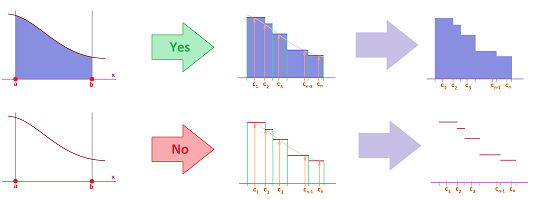
We have successfully used the Riemann sum construction to approximate and, at the limit, compute the areas under the graphs of functions. It would be, however, a grave mistake to think that the step function produced by this construction can serve as an approximation of the function itself.
The reason is revealed when we watch how spectacularly this idea fails when applied to computing the lengths of curves.
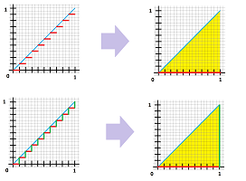
Example. Let's consider a very simple case of $y=f(x)=x$ over $[0,1]$. The approximation of the curve with the horizontal segments looks just as good as the approximation of the area under the graph:
The result is illustrated for a partition with $n=10$ intervals of equal length and the left ends as secondary nodes.
A problem appears when we look at the actual numbers. The length of the original graph is $\sqrt{2}$ by the Pythagorean Theorem. Meanwhile, the total length of the horizontal segments that make up the graph of the resulting step function is $1$; it's simply the bottom of the big triangle. Too low!
One may try to fix the problem by adding the vertical segments to our estimate of the length of the diagonal. Then, the estimate becomes $2$; it's simply the sum of the other two sides of the big triangle. Too high! It is important that the numbers won't change even if we start to refine the partition. In contrast, the approximation of the area of the triangle, $L_n$, is getting better as we increase $n$.
To understand the reason for this discrepancy, let's consider the line $y=g(x)=x/2$. Its actual length is $\sqrt{1^2+(1/2)^2}\approx 1.19$ by the Pythagorean Theorem. The approximation with horizontal segments is still equal to $1$ and the one with both vertical and horizontal segments is $1.5$. The estimates are still off but they are closer to the truth!
What explains the difference? The slope. To confirm this idea, just take the line with zero slope. Then the estimate is equal to its actual length!
In fact, the case of a linear $f$ is very simple: $$\text{Length }=\sqrt{ \text{ base }^2 + \text{ height }^2}=\sqrt{ \text{ base }^2 +\left( \text{ base }\cdot \text{ slope } \right)^2}.$$ $\square$
Exercise. Show that the conclusions remain valid no matter what augmented partition of $[0,1]$ we choose.
Exercise. Show that the length of the graph of a step function over any partition of $[a,b]$ is $b-a$.
The lesson is that the estimate for the length of the graph -- unlike the one for the area under the graph -- should depend on the derivative of the function.
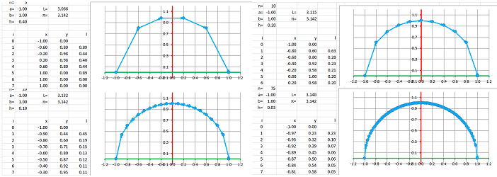
Example. But first, let's compute length of the circle as the graph of a function. We compute the length of the upper half of the unit circle by first representing it as the graph of a simple function: $$f(x)=\sqrt{1-x^2}.$$ The idea is simple: place points on the curve, connect them consecutively by edges, and then approximate the curve with a continuous curve made of these edges. We have a list of the values of $x$ in the first column: $$x_0,x_1,...,x_n,$$ and the list of corresponding values of $y$ in the next column: $$y_0=f(x_0),y_1=f(x_1),...,y_n=f(x_n).$$ In the third column, we compute the lengths of the segments via the Distance Formula: $$l_k=\sqrt{(x_{k+1}-x_k)^2+(y_{k+1}-y_k)^2 }.$$ We use the formula: $$\texttt{=SQRT((RC[-2]-R[-1]C[-2])^2+(RC[-1]-R[-1]C[-1])^2)}.$$
As we increase the number of segments, $n$, the result that we know to be correct, $\pi$, is being approached. We will see in Chapters 14 and 17 a better way to represent curves and especially the circle. $\square$
We will, just as before, use a partition of the interval to split the curve into smaller pieces but then we will approximate these pieces not with horizontal segments but with secant lines.
But we, just as always, start with a discrete situation. We simply have a sequence of points on the plane. Such a square is seen as a “curve” if we proceed from point to point along a straight line. The lengths of these segments are found by the Distance Formula, just as in the above example. It is this simple!
Now, something a bit more specific. What if these points form the graph of a function $y=f(x)$ defined at the nodes of a partition of $[a,b]$?
This is what happens to each interval $[x_{k-1},x_k],\ k=1,2,..., n$ of the partition. The graph of $f$ goes (jumps) from $(x_{k-1},f(x_{k-1}))$ to $(x_k,f(x_k))$. We then construct a sloped segment between these two points:
It is the secant line! A right triangle is formed by these two segments:
- horizontal $[x_{k-1},x_k]$, and
- vertical from $f(x_{k-1})$ to $f(x_k)$, or vice versa.
The lengths of these sides are:
- horizontal (base, the run): $h=x_k-x_{k-1}=\Delta x_k$, and
- vertical (height, the rise): $|f(x_k)-f(x_{k-1})|=\Delta y_k$.
The length of the edge (the hypotenuse of the triangle) is then: $$\sqrt{\Delta x_k^2+\Delta y_k^2}=\sqrt{\Delta x_k^2+(f(x_k)-f(x_{k-1}))^2}.$$ Thus, the full length of the trip along these points on the graph of $f$ is equal to: $$\text{total length }=\sum_{k=1}^n \sqrt{\Delta x_k^2+\Delta y_k^2}=\sum_{k=1}^n\sqrt{\Delta x_k^2+(f(x_k)-f(x_{k-1}))^2}.$$
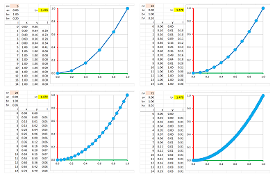
Example. We approximate the length of a parabola $y=x^2,\ 0\le x\le 1$, below:
$\square$
What if now we have a continuous curve, the graph of $y=f(x)$ defined on the whole interval $[a,b]$? These estimates are exact in the case of a linear $f$.
We will, just as before, use a partition of the interval to split the curve into smaller pieces but then we will approximate these pieces not with horizontal segments but with secant lines.
Let's define and then compute the length of the graph of $y=f(x)$ over the interval $[a,b]$.
Then, the full length of the graph of $f$ is approximated by the sum of all $n$ of those, as follows: $$\text{length }\approx L_n=\sum_{k=1}^n\sqrt{\Delta x_k^2+(f(x_k)-f(x_{k-1}))^2}.$$ The limit of this sequence is the meaning of the length of the curve! We would prefer, however, to connect this idea back to idea of Riemann integral and to the machinery that we have developed. Unfortunately, this expression doesn't look like the Riemann sum of a function! What is missing is $\Delta x_k$ as a multiple in each of the terms. We will have to create it by manipulating the formula.
We also use the insight from the earlier discussion: there must be the derivative of $f$ present. This means that we must see the difference quotient in the formula! Where is it? We see the difference but not the difference quotient. We will need to create it by manipulating the formula.
The two goals match up: we divide and multiply each term by $\Delta x_k$, as follows: $$\begin{array}{lll} \text{sum of lengths }&= \sum_{k=1}^n \sqrt{ \Delta x_k^2+(f(x_k)-f(x_{k-1}))^2 }\\ &= \sum_{k=1}^n \sqrt{\Delta x_k^2+(f(x_k)-f(x_{k-1}))^2}\cdot \frac{\Delta x_k}{\Delta x_k}\\ &= \sum_{k=1}^n \sqrt{ \frac{1}{\Delta x_k^2}\left( \Delta x_k^2+(f(x_k)-f(x_{k-1}))^2 \right) }\cdot \Delta x_k &\text{ ...here is }\Delta x_k,\\ &= \sum_{k=1}^n \sqrt{ 1+\left( \frac{f(x_k)-f(x_{k-1})}{\Delta x_k} \right)^2 }\cdot \Delta x_k &\text{ ...here is the difference quotient.} \end{array}$$ But this is still not the Riemann sum... The expression that precedes $h$ should be the value of some function evaluated at the secondary nodes of the partition. We haven't specified those yet and this is the time to do that. We apply, as we've done before, the Mean Value Theorem: there is some $c_k$ in the interval $[x_{k-1},x_k]$ such that the slope of the tangent line at that location is equal to the slope of the secant line over the interval: $$\frac{f(x_k)-f(x_{k-1})}{\Delta x_k}=f'(c_k).$$ Therefore, $$\text{sum of lengths }=\sum_{k=1}^n \sqrt{ 1+\left( f'(c_k) \right)^2 }\cdot \Delta x_k.$$ Finally, this is the Riemann sum of the function $g(x)=\sqrt{ 1+\left( f'(x) \right)^2 }$ over the partition of $[a,b]$ with the secondary nodes $c_1,...,c_n$!
Just as for the area (mass, work, etc.), the analysis above reveals the meaning of the new concept.
Definition. The length of the curve given by the graph $y=f(x)$ of a differentiable function over interval $[a,b]$ is defined to be the integral $$\int_a^b \sqrt{ 1+\left( f' \right)^2 }\, dx,$$ if it exists.
Note that the function $f$ itself is absent from the formula! That's understandable because only the shape (given by the derivative) and not the location that matters for the length of the curve. In fact, we know from Chapter 9 that if $f'=g'$, then $f=g+C$.
Theorem. If the derivative of a function $f$ is continuous, the length of the curve given by the graph $y=f(x)$ over $[a,b]$ is defined.
Proof. We need the extra condition to ensure that the Mean Value Theorem applies and the resulting function is integrable. $\blacksquare$
Example. It is time to prove that the circumference of a circle of radius $R$ is $2\pi R$.
We represent, again, the upper half of the circle by the graph: $$y=f(x)=\sqrt{R^2-x^2}.$$ Then, $$f'(x)=-\frac{x}{\sqrt{R^2-x^2}}.$$ We apply the formula: $$\begin{array}{lll} \text{Half of the length }&=\int_a^b \sqrt{ 1+\left( f'(x) \right)^2 }\, dx\\ &=\int _{-R}^R \sqrt{ 1+\left( -\frac{x}{\sqrt{R^2-x^2}} \right)^2 }\, dx\\ &=\int _{-R}^R \sqrt{ 1+\frac{x^2}{R^2-x^2} }\, dx\\ &=\int _{-R}^R \sqrt{ \frac{R^2}{R^2-x^2} }\, dx\\ &=R\cdot \int _{-R}^R \frac{1}{\sqrt{R^2-x^2}}\, dx\\ &=...\\ &=R\cdot \pi &\text{, via trig substitution.}\\ \end{array}$$ $\square$
Exercise. Find the length of the segment of the parabola $y=x^2$ from $(0,0)$ to $(1,1)$.
Exercise. Find the length of the segment of the curve $y=x^3$ from $(0,0)$ to $(1,1)$.
Exercise. Find the length of the segment of the curve $y=\sin x$ above the interval $[0,\pi]$.
The coordinate system for dimension $3$
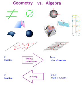
We pursued the idea of a coordinate system in order to transition from
- geometry: points, lines, triangles, circles, planes, cubes, spheres, etc., to
- algebra: numbers, combinations of numbers, functions, etc.
This approach allows us to solve geometric problems -- such as finding the distance between two points -- without measuring.
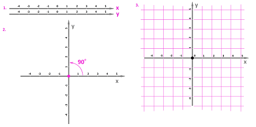
Recall how, for dimension $2$, the coordinate system is built:
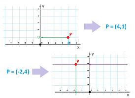
We have a correspondence: $$\begin{array}{|c|}\hline \quad \text{location } P\ \longleftrightarrow\ \text{ pair }\ (x,y) .\quad \\ \hline\end{array}$$ This is how it works:
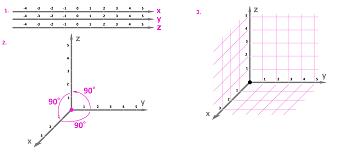
We continue with dimension $3$. There is much more going on:
It is built in several stages:
- 1. three coordinate axes are chosen, the $x$-axis, the $y$-axis, and the $z$-axis;
- 2. the two axes are put together at their origins so that it is a $90$-degree turn from the positive direction of one axis to the positive direction of the next -- from $x$ to $y$ to $z$ to $x$;
- 3. use the marks on the axis to draw a grid.
Alternatively, the system is built from three copies of the Cartesian plane: the $xy$-plane, the $yz$-plane, and the $zx$-plane. They are called the coordinate planes.
We have, as before, a correspondence: $$\begin{array}{|c|}\hline \quad \text{location } P\ \longleftrightarrow\ \text{ triple }\ (x,y,z) .\quad \\ \hline\end{array}$$ that works in both directions.
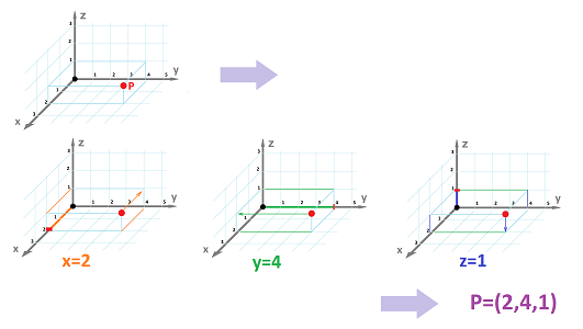
For example, suppose $P$ is a location in this space. We then find the distances from the three planes to that location -- positive in the positive direction and negative in the negative direction -- and the result is the three coordinates of $P$, some numbers $x$, $y$, and $z$. The distance from the $yz$-plane is measured along the $x$-axis, etc. We use the nearest mark to simplify the task.
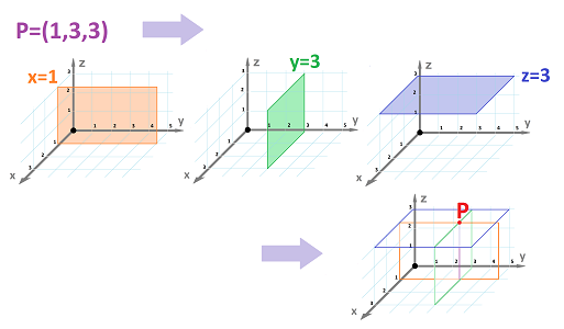
Conversely, suppose $x,y,z$ are numbers.
- First, we measure $x$ as the distance from the $yz$-plane -- positive in the positive direction and negative in the negative direction -- along the $x$-axis and create a plane parallel to the $yz$-plane.
- Second, we measure $y$ as the distance from the $xz$-plane along the $y$-axis and create a plane parallel to the $xz$-plane.
- Third, we measure $z$ as the distance from the $xy$-plane along the $z$-axis and create a plane parallel to the $xy$-plane.
The intersection of these three planes -- as if these were the two walls and the floor in a room -- is a location $P=(x,y,z)$ in the space. We use the nearest marks to simplify the task.
This $3$-dimensional coordinate system is called the Cartesian space or the $3$-space.
Once the coordinate system is in place, it is acceptable to think of location as triples of numbers and vice versa. In fact, we can write: $$P=(x,y,z).$$
One can think of the $3$-space as a stack of planes, each of which is just a copy of one of the coordinate planes:
We can use this idea to reveal the internal structure of the space.
Theorem.
- (a) If $L$ is a plane parallel to the $xy$-plane, then all points on $L$ have the same $z$-coordinate. Conversely, if a collection $L$ of points consists of all points with the same $z$-coordinate, $L$ is a plane parallel to the $xy$-plane.
- (b) If $L$ is a plane parallel to the $yz$-plane, then all points on $L$ have the same $x$-coordinate. Conversely, if a collection $L$ of points consists of all points with the same $x$-coordinate, $L$ is a plane parallel to the $yz$-plane.
- (c) If $L$ is a plane parallel to the $zx$-plane, then all points on $L$ have the same $y$-coordinate. Conversely, if a collection $L$ of points consists of all points with the same $y$-coordinate, $L$ is a plane parallel to the $zx$-plane.
Then, we have a compact way to represent these planes: $$x=k,\ y=k,\ \text{ or } z=k,$$ for some real $k$.
Now that everything is pre-measured we can solve the geometric problems by algebraically manipulating coordinates.
The first geometric task is finding the distance. What is the distance between locations $P$ and $Q$ in terms of their coordinates $(x,y,z)$ and $(x',y',z')$?
For dimension $2$, we used the distance formula from the $1$-dimensional case. We found distance between two points on the plane as the length of the diagonal of the rectangle -- with its sides parallel to the coordinate axes -- that has these points at the opposite corners:
Similarly, we find distance between two points in space as the length of the diagonal of the box -- with its edges parallel to the coordinate axes and sides parallel to the coordinate planes -- that has these points at the opposite corners:
Theorem (Distance Formula for dimension $3$). The distance between points with coordinates $P=(x,y,z)$ and $Q=(x',y',z')$ is $$d(P,Q)=\sqrt{(x-x')^2+(y-y')^2+(z-z')^2}.$$
Proof. We use the distance formula from the $1$-dimensional case separately for each of the three axes, as follows. The distance
- between $x$ and $x'$ on the $x$-axis is $|x-x'|$,
- between $y$ and $y'$ on the $y$-axis is $|y-y'|$, and
- between $z$ and $z'$ on the $z$-axis is $|z-z'|$.
Then, the segment between the points $P=(x,y,z)$ and $Q=(x',y',z')$ is the diagonal of this “box”. Its sides are: $|x-x'|$, $|y-y'|$, and $|z-z'|$. Our conclusion below follows from the Pythagorean Theorem applied twice: we first find the length of the diagonal of the opposite face of the box and then the length of the main diagonal, as follows: $$\begin{array}{lllll} d(P,A)=|x-x'|,& d(A,B)=|y-y'|& \Longrightarrow&d(P,B)^2&=(x-x')^2+(y-y')^2;\\ d(P,B)^2=(x-x')^2+(y-y')^2,& d(B,Q)=|z-z'|& \Longrightarrow &d(P,Q)^2&=d(P,B)^2+d(B,Q)^2\\ &&&&=(x-x')^2+(y-y')^2+(z-z')^2. \end{array}$$ $\blacksquare$
Exercise. Prove that in the latter case the triangle is indeed right.
A treatment of the second geometric task, directions, is postponed until Chapter 16.
Relations are used in the same way as before but with more variables. A relation processes a triple of numbers $(x,y,z)$ as the input and produces an output, which is: Yes or No. If we are to plot the graph of a relation, this output becomes: a point or no point; for example: $$ \newcommand{\ra}[1]{\!\!\!\!\!\xrightarrow{\quad#1\quad}\!\!\!\!\!} \newcommand{\da}[1]{\left\downarrow{\scriptstyle#1}\vphantom{\displaystyle\int_0^1}\right.} % \begin{array}{ccccccccccccccc} \text{input} & & \text{relation} & & \text{output} \\ (x,y,z) & \mapsto & \begin{array}{|c|}\hline\quad x+y+z=2? \quad \\ \hline\end{array} & \ra{Yes} & \text{ plot } (x,y,z)\\ &&\downarrow ^{No}\\ &&\text{ don't plot } \end{array}$$ We can do it by hand:
We can use, as before, the set-building notation: $$\{ (x,y,z):\ \text{ a condition on }x,y,z\}.$$ For example, the graph of the above relation is a subset of ${\bf R}^2$ given by: $$\{ (x,y,z):\ x+y+z=2\}.$$
Example. Let's consider something more complex: $$ \newcommand{\ra}[1]{\!\!\!\!\!\xrightarrow{\quad#1\quad}\!\!\!\!\!} \newcommand{\da}[1]{\left\downarrow{\scriptstyle#1}\vphantom{\displaystyle\int_0^1}\right.} % \begin{array}{ccccccccccccccc} \text{input} & & \text{relation} & & \text{output} \\ (x,y,z) & \mapsto & \begin{array}{|c|}\hline\quad x^2+y^2+z^2=1? \quad \\ \hline\end{array} & \ra{Yes} & \text{ plot } (x,y,z)\\ &&\downarrow ^{No}\\ &&\text{ don't plot } \end{array}$$ We test each of these triples $(x,y,z)$ with the help of a spreadsheet:
How do we plot the graph of this relation? Just as before, instead of testing whether $x^2+y^2+z^2$ is equal to $1$, we check whether it is within a small fixed number, such as $.001$, from $1$ before we plot it. The spreadsheet is evaluated separately for several distinct values of $z$. The result looks like a surface. Indeed, since $x^2+y^2+z^2$ is the square of the distance from $(x,y,z)$ to the origin, we have a sphere. $\square$
Theorem. The sphere of radius $R>0$ centered at point $(h,k,l)$, which is the collection of all points $R$ units away from $(h,k,l)$, is given by the relation: $$(x-h)^2+(y-k)^2+(z-l)^2=R^2.$$
Proof. It follows from the Distance Formula for dimension $3$. $\blacksquare$
Theorem. The cylinder of radius $R>0$ centered around the $z$-axis, which is the collection of all points $R$ units away from the axis measured horizontally, is given by the relation: $$x^2+y^2=R^2.$$
Proof. It follows from the Distance Formula for dimension $2$. $\blacksquare$
Representations of sets of all points $1$ unit away from the origin are presented below, for the dimensions of the space $n=1,2,3$: $$\begin{array}{|r|c|c|c|} \hline \text{dimension:}&1&2&3\\ \hline \text{distance }=1&|x|=1&x^2+y^2=1&x^2+y^2+z^2=1\\ \text{set:}&\text{two points}&\text{circle}&\text{sphere}\\ \text{its “size”:}&&\text{length}&\text{area}\\ \hline \text{distance }\le 1&|x|\le1&x^2+y^2\le1&x^2+y^2+z^2\le1\\ \text{set:}&\text{interval}&\text{disk}&\text{ball}\\ \text{its “size”:}&\text{length}&\text{area}&\text{volume}\\ \hline \end{array}$$ The latter list is a list of the building blocks called “cells”. They are presented below, for the dimensions of the cells $m=0,1,2,3$:
The transition from relations of three variables to functions of two variables will be postponed.
We see how much harder it is to visualize things in the $3$-dimensional space and why it will require a further development of the algebraic treatment of geometry that we have presented. It is presented in Chapter 20.
Volumes via cross-sections
We have come to understand areas in terms of lengths. Indeed, if we rearrange these pencils by moving each up or down, they will still cover the same area:
This fact is meant to illustrate the following situation. Suppose we have four functions $f,g,F,G$ that have nothing to do with each other except the distance between the graphs -- on the $xy$-plane -- is the same: $$f(x)-g(x)=F(x)-G(x),$$ for all $x$ in $[a,b]$. Let's compare: the area between $f$ and $g$ vs. the area between $F$ and $G$. Each pair of corresponding rectangles in the approximations of the two areas over some partition have the same height (same pencil).
That is why the Riemann sums that approximate the areas between either pair of graphs are the same: $$\sum_{[a,b]}(f-g)\, \Delta x=\sum_{[a,b]}(F-G) \, \Delta x,$$ over any augmented partition $P$. Therefore, the integrals -- the areas between the graphs -- are equal too: $$\int_a^b(f-g)\, dx =\int_a^b(F-G)\,dx.$$
Example. The area between the graphs of $y=x^2+1$ and $y=x^2+2$ is the same as that of the square below:
$\square$
Conclusion: a vertical cross-section of this region corresponding to $x$ is the vertical interval $[g(x),f(x)]$ and only its length, $f(x)-g(x)$, affects the area of the region.
Let's now go up in dimensions and examine the cross-sections of solids.
But first, what is volume? The question will be address in full only in Chapter 20. For now, we will rely on a simplifying assumption. We do understand the meaning of the volume of such a simple sold as a box. It is $V=w\cdot d\cdot h$, where $w$ is the width, $d$ the depth, and $h$ the height. We also “know” the volume of the cylinder, $V=\pi R^2 h$, where $R$ is its radius and $h$ is the height.
We can gain insight from this: $$\text{ volume }= \text{ area of the base }\cdot\text{ height }.$$ Indeed, the area of the base is, respectively, $A=wd$ and $A=\pi R^2$. The same is true for the prism.
What do they all have in common? The base is a region on the plane and we might know its area $A$ (following the last section). This region is lifted off the plane to the height $h$. Between these two plane regions lies a cylinder-like solid:
We will assume that its volume is: $$V=A\cdot h.$$
Just as in the last section rectangles were used to approximate the slices of the regions, these “shells” will approximate slices of solids.
Suppose that, instead of a stack of pencils, we have a stack of coins. If we rearrange these coins by moving them side to side, the total volume will remain the same:
We realize that we should try to understand volumes in terms of areas. It is called the Cavalieri principle: $$\begin{array}{ll} \text{ if the vertical cross-sections of two } -\!\!\big \langle \begin{array}{cc}\text{regions in the plane}\\ \text{solids in the space}\end{array} \big \rangle\!\! - \\ \text{ have equal }-\!\!\big \langle \begin{array}{cc}\text{lengths}\\ \text{areas}\end{array}\big \rangle \!\! - \text{, then their } -\!\!\big \langle\begin{array}{cc}\text{areas}\\ \text{volumes}\end{array} \big \rangle\!\! -\text{ are also equal.} \end{array}$$
Suppose our solid $S$ is located in the Cartesian space. Its cross-section are the intersections of $S$ with the various planes, especially the ones parallel to the coordinate plane. We choose those parallel to the $yz$-plane and, therefore, perpendicular to the $x$-axis. Thus, we will consider all vertical cross-section of this solid corresponding to all values $x$ as the intersections of $S$ with the vertical planes through the point $x$ on the $x$-axis. Each of them is the plane region and, according to the Cavalieri principle, only its area affects the volume of the region:
We denote this area by $A(x)$. It is a function of $x$.
Example. What is the volume of the cylinder of radius $R$ and height $h$?
It is located in our $3$-space, but all we need to know is its dimensions. We have $$A(x)=\pi R^2.$$ By the Cavalieri principle, the volume of this cylinder is the same as the volume of a box the cross-section of which is a square with area $\pi R^2$ and the same height: $$\text{Volume }=\pi R^2 \cdot h.$$ $\square$
Let's confirm the idea of the Cavalieri principle via Riemann sums.
We place the $x$-axis somehow along the solid. Suppose the solid $S$ lies entirely between some vertical planes $x=a$ and $x=b$. We continue with an augmented partition $P$ of the interval $[a,b]$: $$a=x_0\le c_1\le x_1\le ... \le x_n=b.$$ The vertical planes $x=x_i$ cut the solid into $n$ slices. The $i$th slice is approximated by the following. The cross-section of $S$ created by the vertical plane $x=c_i$ is a plane region; its area is $A(c_i)$:
We construct a new solid from this plane region by giving it a thickness equal to $\Delta x_i=x_i-x_{i-1}$. Then its volume is $A(c_i)\cdot\Delta x_i$. The total volume of these solids is equal to: $$\sum _{i=1}^n A(c_i)\, \Delta x_i = \sum_{[a,b]} A\, \Delta x,$$ and it is then recognized as the Riemann sum of $y=A(x)$ over $[a,b]$.
Definition. The volume of a solid is defined to be the integral $$\int_a^b A(x)\, dx,$$ if it exists, where $A(c)$ is the area (if it exists) of the intersection of the solid and the plane $x=c$.
Note that the area $A(x)$ itself, for each $x$, is understood, and may have to be computed, as a Riemann integral.
Thus, the volume is the integral of the area:
Example. The cross-sections of the sphere are circles:
More precisely, the cross-sections of the ball are disks and it is the areas of these disks that we need to find. Suppose the radius of this circle at $x$ is $r$. What is it? Let's take a side view:
Then $$x^2+r^2=R^2.$$ Then the area of this circle is: $$A(x)=\pi \left(\sqrt{R^2-x^2}\right)^2=\pi (R^2-x^2);$$ therefore, $$\text{Volume }=\int_{-R}^R A(x)\, dx=\pi\int_{-R}^R \left( R^2-x^2 \right)\, dx=\pi \left(R^2x-\frac{1}{3}x^3 \right)\Bigg|_{-R}^R=\frac{4}{3}\pi R^3.$$ $\square$
What if the cross-sections are circles but they change from slice to slice? We have done all preliminary work!
Definition. Suppose $y=f(x)$ satisfy $f(x)\ge 0$ for all $x$ in $[a,b]$. Then, the solid of revolution of $f$ about the $x$-axis is the set in the $xyz$-space: $$\{(x,y,z):\ \sqrt{y^2+z^2}\le f(x)\}.$$
Theorem. Suppose $y=f(x)$ satisfy $f(x)\ge 0$ for all $x$ in $[a,b]$. Then, the volume of the solid of revolution of $f$ about the $x$-axis is: $$V=\int_a^b\pi f(x)^2\, dx.$$
Exercise. Prove the theorem.
Warning: even when the cross-sections are circles, they may change from slice to slice in ways that are so complex that we may have to turn to numerical integration.
In general, cross-sections can have any geometry or topology:
Exercise. Describe the cross-sections of these surfaces.
Example. Let's find the volume of the right (i.e., one with its height perpendicular to its base) pyramid with square base with side $2h$ and height $h$. Its cross-sections parallel to the base are squares:
The side of the square located $x$ units from the base is $2(h-x)$; therefore, $$\text{Volume }=\int_{0}^h A(x)\, dx=\int_{0}^h 2(h-x)^2 \, dx= -\frac{2}{3}(h-x)^3 \Bigg|_{0}^h=\frac{2}{3} h^3.$$ $\square$
Exercise. Modify the above example to find the volume of the right pyramid with square base with side $Q$ and height $h$.
Exercise. Find the volume of the right cone with a circular base of radius $R$ and height $h$.
We defined in this section the volume of a solid via its cross-sections. The definition relies on the cylindrical slices to approximate the solid. These complex objects are to be replaced with true elementary building blocks of solids: bricks and boxes. The general definition is presented in Chapter 20.
Exercise. (a) Prove that the work needed to fill -- from the bottom -- a tank located between the planes $x=0$ and $x=h$ (the $x$-axis is vertical) and with the area of its horizontal cross section at height $x$ equal to $A(x)$ is $\int_0^h A(x)x\, dx$. (b) Show that this work is equal to the work needed to move this mass from height $0$ to the height of the center of mass of the tank.
Exercise. Set up but do not evaluate the Riemann sums and the integral for the volume of a box $W\times D\times H$ in terms of its cross-sections.
Volumes of solids of revolution
Suppose we have an object that is rotated as it hardens.
The same effect is produced by using a cutting tool on a hard object as it is being rotated.
Let's rotate a curve. If this curve is a circle, the result of the rotation is similar to a slinky:
Mathematically, we have a curve and a line on the $xy$-plane, we add the $z$-axis, then we rotate the curve around the line in the resulting $3$-space, one point at a time.
Each of the points on the curve produces a circle. Together these circles form a surface. This surface bounds a solid. What is the volume of this solid?
Suppose this curve is simply the graph of a function $$y=f(x)\ge 0,\ a\le x\le b,$$ and suppose the line is the $x$-axis or the $y$-axis:
As the choice of the $x$-axis is easily addressed by the Cavalieri principle, we choose the $y$-axis.
Let's be clear what we are talking about. The surface created by a rotated curve has no volume; the solid it -- partially -- bounds does. For the case of a decreasing $f$, this solid contains every point $(x,y,z)$ that satisfy:
- its distance (measured horizontally) from the $y$-axis is between $a$ and $x$ units,
- its distance (measured vertically) from the $xz$-plane is between $f(b)$ and $f(x)$ units.
Exercise. Describe the solid for the case of an increasing $f$.
The analysis of the idea of volume following the Cavalieri principle is based on cutting the solid into disks. Of course, it can be used for either case. Instead, we start from scratch and pursue the idea of cutting the solid into washers (rings).
We will use, however, the following fact previously derived from the Cavalieri principle.
Proposition. The volume of a washer with the inner radius $r$, the outer radius $R$, and thickness $h$ is the difference of the volumes of the two cylinders: $$\text{volume }=\pi R^2h-\pi r^2h=\pi h(R^2-r^2).$$
Example. Suppose the object is simply the combination of a disk of radius $1$ and the washer around it of thickness $1$:
Then, the volume is simply the sum of the volume of the disk and the volume of the washer: $$\begin{array}{lll} \text{volume }&=2\cdot\text{area of the disk }&+ 1\cdot\text{area of the washer }\\ &=2\cdot \pi \cdot 1^2 &+1\cdot (\pi \cdot 2^2-\pi \cdot 1^2). \end{array}$$ $\square$
Example. Suppose the thickness is changing linearly: from $1$ to $2$.
What is the volume of this object? Even though we know the answer from the Cavalieri principle, we will have to start with approximations again... $\square$
We have an augmented partition $P$ of the radius: $$a=x_0\le c_1\le x_1\le ... \le c_n\le x_n=b,$$ with these lengths of segments: $$\Delta x_i=x_i-x_{i-1}.$$ Here, we cut the solid into thin washers by the cylinders starting at points $x=x_i$ on the $x$-axis and then sample its height at the points $c_i$:
Then the height of each washer $f(c_i)$ and we have: $$\text{mass of }i\text{th washer }= \text{radius}\cdot \text{area}=f(c_i)\cdot\left( \pi x_i^2 -\pi x_{i-1}^2 \right),$$ since the inside radius of the washer is $x_{i-1}$ and the outside is $x_i$.
Then, $$\text{total volume }= \sum_{i=1}^n f(c_i)\cdot \pi\left( x_i^2 -x_{i-1}^2 \right).$$ We can use this formulas for computations.
What is the solid isn't actually made of washers and its thickness varies continuously?
Then the volume of each washer -- when thin enough -- is approximated by the volume of such a washer with the constant height $f(c_i)$: $$\text{mass of }i\text{th washer }\approx \text{radius}\cdot \text{area}=f(c_i)\cdot\left( \pi x_i^2 -\pi x_{i-1}^2 \right).$$ Then, $$\text{total volume }\approx \sum_{i=1}^n f(c_i)\cdot \pi\left( x_i^2 -x_{i-1}^2 \right).$$ This is the volume of the washers built on top of the augmented partition. This time, however, we do not recognize this expression as the Riemann sum of the function over this partition, which is $\sum_{i=1}^n f(c_i)\cdot \Delta x_i$. Is it the Riemann sum of another function? Let's see: $$\text{total volume }\approx \sum_{i=1}^n \pi f(c_i)(x_i+x_{i-1})\cdot \Delta x_i.$$ We need to do something about the term $(x_i+x_{i-1})$...
We back up a bit. Let's assume that function $f$ is integrable. Then the choice of secondary nodes is ours. Let's choose the mid-points: $$c_i=\frac{1}{2}(x_i+x_{i-1}).$$ Then, $$\text{total volume }\approx 2\pi \sum_{i=1}^n f(c_i)c_i\cdot \Delta x_i.$$ This time, we do recognize this expression as the Riemann sum of a simple function. Then, we define the volume of the solid as the limit of these Riemann sums; i.e., $$\text{volume }=2\pi\int_a^b xf(x)\, dx.$$ The limit exists because $xf(x)$ is integrable by the Product Rule. We call this the volume of the solid of revolution obtained by rotating of the graph of $f$.
It is important to confirm that this new definition of volume matches the old one.
Theorem. Given an integrable function $f$ on segment $[a,b]$, the above integral is equal to the volume of the solid of revolution obtained by rotating of the graph of $f$: $$\text{volume }=2\pi\int_a^b xf(x)\, dx.$$
Proof. For simplicity, we assume that $f$ is decreasing. We start with the definition of volume of the Cavalieri principle. The cross-sections of the solid along the $y$-axis are circles; specifically, the intersection of the surface with the plane $y=q$ is a circle of radius $f^{-1}(q)$.
Let's consider the whole solid swept by this curve. We know this: $$\text{volume }=\pi\int_{f^{-1}(b)}^{f^{-1}(a)}\left( f^{-1}(y) \right)^2\, dy.$$ We apply Integration by Substitution with $x=f^{-1}(y)$. Then, $$\text{volume }=\pi\int_{b}^{a}x^2f'(x)\, dx.$$ We apply Integration by Parts with $u=x^2,\ dv = f'\, dx$. Then, $$\begin{array}{ll} \text{volume }&=\pi\left( x^2f(x)\Bigg|_b^a-\int_{b}^{a}2xf(x)\, dx \right)\\ &=\pi a^2f(a)-\pi b^2f(b)+2\pi\int_{a}^{b}xf(x)\, dx. \end{array}$$ The extra terms come from the disk at the bottom and the cylinder in the middle to be removed:
$\blacksquare$
Exercise. Modify the proof of the theorem for the case of an increasing $f$.
